Orion1

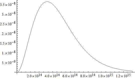
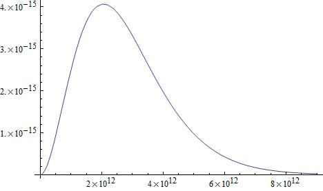
\[\color{blue}{\text{Toy model quantum particle properties chart:}}\] \[\begin{array}{l*{9}{c}r} & \text{identity} & \text{helicity state} & \text{spin} & n_{s} & N_{s} & N_{n} & \text{mass} & \text{type} & \text{spectral radiance peak frequency} \\ b & \text{quinton} & 0 & 0 & 1 & 1 & 1 & 0 & \Lambda & 2.058 \; \text{THz} \\ b & \text{scalaron} & 0 & 0 & 1 & 1 & 1 & 18.658 \; \text{eV} & \phi & 114.366 \; \text{GHz} \\ f & \text{sterile neutrino} & +,- & 1/2 & 2 & 3 & 3 & 8.167 \; \text{eV} & \nu_{s} & 126.915 \; \text{GHz} \\ f & \text{neutrino} & +,- & 1/2 & 2 & 3 & 3 & 0.038 \; \text{eV} & \nu & 126.915 \; \text{GHz} \\ b & \text{photon} & +,- & 1 & 2 & 1 & 2 & 0 & \gamma & 160.229 \; \text{GHz} \\ b & \text{graviton} & +,- & 2 & 2 & 1 & 2 & 0 & \text{G} & 114.366 \; \text{GHz} \\ \end{array}\] \[\color{blue}{\text{Planck's law:}} \; (\color{blue}{\text{ref. 1}})\] \[B\left(f_{\gamma},T_{\gamma} \right) = \frac{N_{\gamma} h f_{\gamma}^{3}}{c^{2} \left(e^{\frac{h f_{\gamma}}{k_{B} T_{\gamma}}} \pm 1 \right)}\] \[\color{blue}{\text{A plus sign in the denominator is a Fermi-Dirac distribution, a minus sign in the denominator is a Bose-Einstein distribution.}}\] \[\color{blue}{\text{+ sign - Fermi-Dirac distribution}}\] \[\color{blue}{\text{- sign - Bose-Einstein distribution}}\] \[\color{blue}{\text{Planck's law energy distribution frequency plot.}} \; (\color{blue}{\text{attached graph 1}})\] \[114.366 \; \text{GHz} \; \; \; 126.915 \; \text{GHz} \; \; \; 160.229 \; \text{GHz}\] \[\color{blue}{\text{Planck's law energy distribution frequency plot.}} \; (\color{blue}{\text{attached graph 2}})\] \[2.058 \; \text{THz}\] \[\color{blue}{\text{In this toy model, some quantum particle radiation distributions are embedded within the photon radiation distribution.}}\] \[\color{blue}{\text{Would a quantum particle radiation distribution embedded within the photon radiation distribution induce cosine anisotropy in the photon radiation?}} \; (\color{blue}{\text{ref. 2}})\] \[\color{blue}{\text{If cosine anisotropy is a detectable amount, is it possible to map cosine anisotropy amounts verses frequency within the photon radiation distribution?}} \; (\color{blue}{\text{ref. 2}})\] \[\color{blue}{\text{Based upon the frequency multi-distribution plot, what frequency domain in the photon radiation distribution would you expect to detect cosine anisotropy?}}\] \[\color{blue}{\text{Any discussions and/or peer reviews about this specific topic thread?}}\] Reference: Wikipedia - Planck's law: (ref. 1) https://en.wikipedia.org/wiki/Planck's_law Wikipedia - Anisotropy - Physics: (ref. 2) https://en.wikipedia.org/wiki/Anisotropy#Physics

...

\[\color{blue}{\text{Symbolic identity key:}}\] \[\begin{array}{lcl} \text{s} \text{ - spin quantum number} \\ n_{s} \text{ - spin states total integer helicity number} \\ N_{s} \text{ - species total integer number} \\ N_{n} \text{ - total effective degeneracy number} \\ \end{array}\] \[n_{s} = 2 s + 1 \; \; \; \; \; \; s < 2 \; \; \; \; \; \; m = 0\] \[n_{s} = 2 \; \; \; \; \; \; s \geq 2 \; \; \; \; \; \; m = 0\] \[\text{if } n_{s} \geq N_{s} \text{ then } N_{n} = n_{s}\] \[\text{if } n_{s} \leq N_{s} \text{ then } N_{n} = N_{s}\] \[\color{blue}{\text{Toy model quantum particle properties chart:}}\] \[\begin{array}{l*{9}{c}r} & \text{identity} & \text{helicity state} & \text{spin} & n_{s} & N_{s} & N_{n} & \text{mass} & \text{type} & \text{spectral radiance peak frequency} \\ b & \text{quinton} & 0 & 0 & 1 & 1 & 1 & 0 & \Lambda & 2.058 \; \text{THz} \\ b & \text{scalaron} & 0 & 0 & 1 & 1 & 1 & 18.658 \; \text{eV} & \phi & 114.366 \; \text{GHz} \\ f & \text{sterile neutrino} & +,- & 1/2 & 2 & 3 & 3 & 8.167 \; \text{eV} & \nu_{s} & 126.915 \; \text{GHz} \\ f & \text{neutrino} & +,- & 1/2 & 2 & 3 & 3 & 0.038 \; \text{eV} & \nu & 126.915 \; \text{GHz} \\ b & \text{photon} & +,- & 1 & 2 & 1 & 2 & 0 & \gamma & 160.229 \; \text{GHz} \\ b & \text{graviton} & +,- & 2 & 2 & 1 & 2 & 0 & \text{G} & 114.366 \; \text{GHz} \\ \end{array}\] \[\color{blue}{\text{For massless quantum particles, the transverse modes cannot exist due to Lorentz invariance.}}\] \[\color{blue}{\text{Only positive and negative helicity states remain. For massless scalar particles, only zero helicity states remain.}}\] \[\color{blue}{\text{The spin 1 photon is also restricted to its positive and negative helicity states, and has a total effective degeneracy number of 2.}}\] \[\color{blue}{\text{A massless graviton has only 2 helicity states, and has a total effective degeneracy number of 2.}}\] \[\color{blue}{\text{Dark energy quinton total effective degeneracy number:}}\] \[\boxed{N_{\Lambda} = 1}\] \[\color{blue}{\text{Planck satellite dark energy cosmological composition parameter:} \; (\text{ref. 1, pg. 11})}\] \[\Omega_{\Lambda} = 0.6825\] \[\color{blue}{\text{Bose-Einstein dark energy cosmic quinton background radiation temperature:} \; (\text{ref. 2})}\] \[\boxed{T_{\Lambda} = \frac{}{k_{B}} \left(\frac{45 \Omega_{\Lambda} H_0^2 \hbar^3 c^5}{4 G N_{\Lambda} \pi^3} \right)^{1/4}}\] \[\boxed{T_{\Lambda} = 35.013 \; \text{K}}\] \[\color{blue}{\text{Bose-Einstein dark energy cosmic quinton background radiation spectral radiance peak frequency:}}\] \[\boxed{f_{\Lambda} = \frac{\left[W_{0}\left(-\frac{3}{e^3} \right) + 3 \right] k_B T_{\Lambda}}{h}}\] \[W_{0}\left(z \right) - \text{Lambert W function} \; \left(\text{ref. 3} \right)\] \[\boxed{f_{\Lambda} = \frac{\left[W_{0}\left(-\frac{3}{e^3} \right) + 3 \right]}{2 \pi} \left(\frac{45 \Omega_{\Lambda} H_0^2 c^5}{4 \hbar G N_{\Lambda} \pi^3} \right)^{1/4}}\] \[\boxed{f_{\Lambda} = 2.05837 \cdot 10^{12} \; \text{Hz}}\] \[\boxed{f_{\Lambda} = 2.058 \; \text{THz}}\] \[\color{blue}{\text{Cosmic photon background radiation temperature at present time:} \; (\text{ref. 4})}\] \[T_{\gamma} = 2.72548 \; \text{K}\] \[\color{blue}{\text{Cosmic neutrino and sterile neutrino background radiation temperature at present time:} \; (\text{ref. 5})}\] \[T_{\nu} = \left(\frac{4}{11} \right)^{\frac{1}{3}} T_{\gamma} = 1.945 \; \text{K}\] \[\boxed{T_{\nu} = 1.945 \; \text{K}}\] \[\color{blue}{\text{Dark matter scalaron and sterile neutrino radiation temperature is equivalent to cosmic neutrino background radiation temperature:}}\] \[\boxed{T_{\phi} = T_{s \nu} = T_{\nu} = 1.945 \; \text{K}}\] \[\color{blue}{\text{Bose-Einstein dark matter cosmic scalaron background radiation spectral radiance peak frequency:}}\] \[\boxed{f_{\phi} = \frac{\left[W_{0}\left(-\frac{3}{e^3} \right) + 3 \right] k_B T_{\phi}}{h}}\] \[W_{0}\left(z \right) - \text{Lambert W function} \; \left(\text{ref. 3} \right)\] \[\boxed{f_{\phi} = 1.14366 \cdot 10^{11} \; \text{Hz}}\] \[\boxed{f_{\phi} = 114.366 \; \text{GHz}}\] \[\color{blue}{\text{Fermi-Dirac dark matter sterile neutrino background radiation spectral radiance peak frequency:}}\] \[\boxed{f_{s \nu} = \frac{\left[W_{0}\left(\frac{3}{e^3} \right) + 3 \right] k_B T_{\nu}}{h}}\] \[W_{0}\left(z \right) - \text{Lambert W function} \; \left(\text{ref. 3} \right)\] \[\boxed{f_{s \nu} = 1.26915 \cdot 10^{11} \; \text{Hz}}\] \[\boxed{f_{s \nu} = 126.915 \; \text{GHz}}\] \[\color{blue}{\text{Solve for cosmic neutrino background radiation spectral radiance peak frequency:}}\] \[\color{blue}{\text{Neutrino species total effective degeneracy number:}}\] \[N_{\nu} = 3.046\] \[\color{blue}{\text{Neutrino radiation energy density Fermi-Dirac distribution:}}\] \[\epsilon_{\nu} = \frac{4 \pi N_{\nu} \left(k_B T_{\nu} \right)^4}{\left(2 \pi \hbar c \right)^3} \int_{0}^c \frac{E_t \left(v \right)^3}{e^{\frac{E_t \left(v \right)}{E_1 \left(T_{\nu} \right)}} + 1} dv\] \[\color{blue}{\text{Solve Fermi-Dirac distribution first derivative x-axis zero intercept with respect to frequency:}}\] \[\frac{d \epsilon_{\nu}}{df_{\nu}} = \frac{d}{df_{\nu}} \left(\frac{4 \pi N_{\nu} \left(k_B T_{\nu} \right)^4 E_t\left(\omega \right)^3}{\left(2 \pi \hbar c \right)^3 \left(e^{\frac{E_t \left(\omega \right)}{E_1 \left(T_{\nu} \right)}} + 1 \right)} \right) = 0\] \[\frac{d}{df_{\nu}} \left(\frac{4 \pi N_{\nu} \left(k_B T_{\nu} \right)^4 \left(h f_{\nu} \right)^3 }{\left(h c \right)^3 \left(e^{\frac{h f}{k_{B} T_{\nu}}} + 1 \right)} \right) = \frac{12 \pi N_{\nu} f_{\nu}^2 \left(k_B T_{\nu} \right)^4}{c^3 \left(e^{\frac{h f_{\nu}}{k_B T_{\nu}}} + 1 \right)} - \frac{4 \pi h N_{\nu} f_{\nu}^3 \left(k_B T_{\nu} \right)^3 e^{\frac{h f_{\nu}}{k_B T_{\nu}}}}{c^3 \left(e^{\frac{h f_{\nu}}{k_B T_{\nu}}} + 1 \right)^2} = 0\] \[\frac{12 \pi N_{\nu} f_{\nu}^2 \left(k_B T_{\nu} \right)^4}{c^3 \left(e^{\frac{h f_{\nu}}{k_B T_{\nu}}} + 1 \right)} = \frac{4 \pi h N_{\nu} f_{\nu}^3 \left(k_B T_{\nu} \right)^3 e^{\frac{h f_{\nu}}{k_B T_{\nu}}}}{c^3 \left(e^{\frac{h f_{\nu}}{k_B T_{\nu}}} + 1 \right)^2}\] \[\frac{h f_{\nu}}{k_B T_{\nu}} = 3 \left(1 + \frac{1}{e^{\frac{h f_{\nu}}{k_B T_{\nu}}}} \right) \; \; \; \; \; \; \frac{h f_{\nu}}{k_B T_{\nu}} = 3 + \frac{3}{e^{\frac{h f_{\nu}}{k_B T_{\nu}}}} \; \; \; \; \; \; \frac{h f_{\nu}}{k_B T_{\nu}} = \frac{3}{e^{\frac{h f_{\nu}}{k_B T_{\nu}}}} + 3\] \[\pm x = \left(y \pm a \right) e^{y} \; \; \; \; \; \; y = \frac{x}{e^{y}} + a \; \; \; \; \; \; y = W_{k}\left(\frac{x}{e^{a}} \right) + a \; \; \; \; \; \; x = 3 \; \; \; a = 3 \; \; \; k = 0\] \[f_{\nu} = \frac{\left[W_{0}\left(\frac{3}{e^3} \right) + 3 \right] k_B T_{\nu}}{h} = 1.26915 \cdot 10^{11} \; \text{Hz} = 126.915 \; \text{GHz}\] \[W_{0}\left(z \right) - \text{Lambert W function} \; \left(\text{ref. 3} \right)\] \[\color{blue}{\text{Fermi-Dirac cosmic neutrino background radiation spectral radiance peak frequency:}}\] \[\boxed{f_{\nu} = \frac{\left[W_{0}\left(\frac{3}{e^3} \right) + 3 \right] k_B T_{\nu}}{h}}\] \[\boxed{f_{\nu} = 1.26915 \cdot 10^{11} \; \text{Hz}}\] \[\boxed{f_{\nu} = 126.915 \; \text{GHz}}\] \[\color{blue}{\text{Solve for cosmic photon background radiation spectral radiance peak frequency:}}\] \[\color{blue}{\text{Photon species total effective degeneracy number:}}\] \[\boxed{N_{\gamma} = 2}\] \[\color{blue}{\text{Cosmic photon background radiation temperature at present time:} \; (\text{ref. 4})}\] \[T_{\gamma} = 2.72548 \; \text{K}\] \[\color{blue}{\text{Planck's law:} \; (\text{ref. 6})}\] \[B\left(f_{\gamma},T_{\gamma} \right) = \frac{N_{\gamma} h f_{\gamma}^{3}}{c^{2} \left(e^{\frac{h f_{\gamma}}{k_{B} T_{\gamma}}} - 1 \right)}\] \[\color{blue}{\text{Solve Bose-Einstein Planck's law first derivative x-axis zero intercept with respect to frequency:}}\] \[\frac{dB\left(f_{\gamma},T_{\gamma} \right)}{df_{\gamma}} = \frac{d}{df_{\gamma}} \left[\frac{N_{\gamma} h f_{\gamma}^{3}}{c^{2} \left(e^{\frac{h f_{\gamma}}{k_{B} T_{\gamma}}} - 1 \right)} \right] = 0\] \[\color{blue}{\text{Planck's law first derivative with respect to frequency:}}\] \[\frac{dB\left(f_{\gamma},T_{\gamma} \right)}{df_{\gamma}} = \frac{d}{df_{\gamma}} \left[\frac{N_{\gamma} h f_{\gamma}^{3}}{c^{2} \left(e^{\frac{h f_{\gamma}}{k_{B} T_{\gamma}}} - 1 \right)} \right] = \frac{3 N_{\gamma} h f_{\gamma}^2}{c^2 \left(e^{\frac{h f_{\gamma}}{k_B T_{\gamma}}} - 1 \right)} - \frac{N_{\gamma} h^2 f_{\gamma}^3 e^{\frac{h f_{\gamma}}{k_B T_{\gamma}}}}{c^2 k_B T_{\gamma} \left(e^{\frac{h f_{\gamma}}{k_B T_{\gamma}}} - 1 \right)^2} = 0\] \[\frac{3 N_{\gamma} h f_{\gamma}^2}{c^2 \left(e^{\frac{h f_{\gamma}}{k_B T_{\gamma}}} - 1 \right)} = \frac{N_{\gamma} h^2 f_{\gamma}^3 e^{\frac{h f_{\gamma}}{k_B T_{\gamma}}}}{c^2 k_B T_{\gamma} \left(e^{\frac{h f_{\gamma}}{k_B T_{\gamma}}} - 1 \right)^2}\] \[\frac{h f_{\gamma}}{k_B T_{\gamma}} = 3 \left(1 - \frac{1}{e^{\frac{h f_{\gamma}}{k_B T_{\gamma}}}} \right) \; \; \; \; \; \; \frac{h f_{\gamma}}{k_B T_{\gamma}} = 3 - \frac{3}{e^{\frac{h f_{\gamma}}{k_B T_{\gamma}}}} \; \; \; \; \; \; \frac{h f_{\gamma}}{k_B T_{\gamma}} = -\frac{3}{e^{\frac{h f_{\gamma}}{k_B T_{\gamma}}}} + 3\] \[\pm x = \left(y \pm a \right) e^{y} \; \; \; \; \; \; y = -\frac{x}{e^{y}} + a \; \; \; \; \; \; y = W_{k}\left(-\frac{x}{e^{a}} \right) + a \; \; \; \; \; \; x = -3 \; \; \; a = 3 \; \; \; k = 0\] \[f_{\gamma} = \frac{\left[W_{0}\left(-\frac{3}{e^3} \right) + 3 \right] k_B T_{\gamma}}{h} = 1.60229 \cdot 10^{11} \; \text{Hz} = 160.229 \; \text{GHz}\] \[W_{0}\left(z \right) - \text{Lambert W function} \; \left(\text{ref. 3} \right)\] \[\color{blue}{\text{Bose-Einstein cosmic photon background radiation spectral radiance peak frequency:}}\] \[\boxed{f_{\gamma} = \frac{\left[W_{0}\left(-\frac{3}{e^3} \right) + 3 \right] k_B T_{\gamma}}{h}}\] \[\boxed{f_{\gamma} = 1.60229 \cdot 10^{11} \; \text{Hz}}\] \[\boxed{f_{\gamma} = 160.229 \; \text{GHz}}\] \[\color{blue}{\text{Observed cosmic photon background radiation spectral radiance peak frequency:} \; (\text{ref. 4})}\] \[f_{\gamma} = 160.23 \; \text{GHz}\] \[\color{blue}{\text{Solve for cosmic photon background radiation spectral radiance peak frequency:}}\] \[\color{blue}{\text{Photon radiation energy density Bose-Einstein distribution:}}\] \[\epsilon_{\gamma} = \frac{4 \pi N_{\gamma} \left(k_B T_{\gamma} \right)^4}{\left( 2 \pi \hbar c \right)^3} \int_{0}^\infty \frac{E_t \left(\omega \right)^3}{e^{\frac{E_t \left(\omega \right)}{E_1 \left(T_{\gamma} \right)}} - 1} d \omega\] \[\color{blue}{\text{Solve Bose-Einstein distribution first derivative x-axis zero intercept with respect to frequency:}}\] \[\frac{d \epsilon_{\gamma}}{df_{\gamma}} = \frac{d}{df_{\gamma}} \left(\frac{4 \pi N_{\gamma} \left(k_B T_{\gamma} \right)^4 E_t\left(\omega \right)^3}{\left(2 \pi \hbar c \right)^3 \left(e^{\frac{E_t \left(\omega \right)}{E_1 \left(T_{\gamma} \right)}} - 1 \right)} \right) = 0\] \[\frac{d}{df_{\gamma}} \left(\frac{4 \pi N_{\gamma} \left(k_B T_{\gamma} \right)^4 \left(h f_{\gamma} \right)^3 }{\left(h c \right)^3 \left(e^{\frac{h f}{k_{B} T_{\gamma}}} - 1 \right)} \right) = \frac{12 \pi N_{\gamma} f_{\gamma}^2 \left(k_B T_{\gamma} \right)^4}{c^3 \left(e^{\frac{h f_{\gamma}}{k_B T_{\gamma}}} - 1 \right)} - \frac{4 \pi h N_{\gamma} f_{\gamma}^3 \left(k_B T_{\gamma} \right)^3 e^{\frac{h f_{\gamma}}{k_B T_{\gamma}}}}{c^3 \left(e^{\frac{h f_{\gamma}}{k_B T_{\gamma}}} - 1 \right)^2} = 0\] \[\frac{12 \pi N_{\gamma} f_{\gamma}^2 \left(k_B T_{\gamma} \right)^4}{c^3 \left(e^{\frac{h f_{\gamma}}{k_B T_{\gamma}}} - 1 \right)} = \frac{4 \pi h N_{\gamma} f_{\gamma}^3 \left(k_B T_{\gamma} \right)^3 e^{\frac{h f_{\gamma}}{k_B T_{\gamma}}}}{c^3 \left(e^{\frac{h f_{\gamma}}{k_B T_{\gamma}}} - 1 \right)^2}\] \[\frac{h f_{\gamma}}{k_B T_{\gamma}} = 3 \left(1 - \frac{1}{e^{\frac{h f_{\gamma}}{k_B T_{\gamma}}}} \right) \; \; \; \; \; \; \frac{h f_{\gamma}}{k_B T_{\gamma}} = 3 - \frac{3}{e^{\frac{h f_{\gamma}}{k_B T_{\gamma}}}} \; \; \; \; \; \; \frac{h f_{\gamma}}{k_B T_{\gamma}} = -\frac{3}{e^{\frac{h f_{\gamma}}{k_B T_{\gamma}}}} + 3\] \[\pm x = \left(y \pm a \right) e^{y} \; \; \; \; \; \; y = -\frac{x}{e^{y}} + a \; \; \; \; \; \; y = W_{k}\left(-\frac{x}{e^{a}} \right) + a \; \; \; \; \; \; x = -3 \; \; \; a = 3 \; \; \; k = 0\] \[f_{\gamma} = \frac{\left[W_{0}\left(-\frac{3}{e^3} \right) + 3 \right] k_B T_{\gamma}}{h} = 1.60229 \cdot 10^{11} \; \text{Hz} = 160.229 \; \text{GHz}\] \[W_{0}\left(z \right) - \text{Lambert W function} \; \left(\text{ref. 3} \right)\] \[\color{blue}{\text{Bose-Einstein cosmic photon background radiation spectral radiance peak frequency:}}\] \[\boxed{f_{\gamma} = \frac{\left[W_{0}\left(-\frac{3}{e^3} \right) + 3 \right] k_B T_{\gamma}}{h}}\] \[\boxed{f_{\gamma} = 1.60229 \cdot 10^{11} \; \text{Hz}}\] \[\boxed{f_{\gamma} = 160.229 \; \text{GHz}}\] \[\color{blue}{\text{Observed cosmic photon background radiation spectral radiance peak frequency:} \; (\text{ref. 4})}\] \[f_{\gamma} = 160.23 \; \text{GHz}\] \[\color{blue}{\text{Cosmic graviton background radiation temperature is equivalent to cosmic neutrino background radiation temperature:}}\] \[\boxed{T_{G} = T_{\nu} = 1.945 \; \text{K}}\] \[\color{blue}{\text{Bose-Einstein cosmic graviton background radiation spectral radiance peak frequency:}}\] \[\boxed{f_{G} = \frac{\left[W_{0}\left(-\frac{3}{e^3} \right) + 3 \right] k_B T_{G}}{h}}\] \[W_{0}\left(z \right) - \text{Lambert W function} \; \left(\text{ref. 3} \right)\] \[\boxed{f_{G} = 1.14366 \cdot 10^{11} \; \text{Hz}}\] \[\boxed{f_{G} = 114.366 \; \text{GHz}}\] \[\color{blue}{\text{Are Fermilab quantum particle detectors capable of detecting cold dark matter quantum particles?} \; (\text{ref. 7})}\] \[\color{blue}{\text{Any discussions and/or peer reviews about this specific topic thread?}}\] Reference: Planck 2013 results. XVI. Cosmological parameters: (ref. 1) http://www.ymambrini.com/My_World/Articles_files/Planck_2013_results_16.pdf Science Forums - Dark energy quinton radiation temperature - Orion1: (ref. 2) https://www.scienceforums.net/topic/86694-observable-universe-mass/?do=findComment&comment=931225 Wikipedia - Lambert W function: (ref. 3) https://en.wikipedia.org/wiki/Lambert_W_function Wikipedia - Cosmic microwave background - Importance of precise measurement: (ref. 4) https://en.wikipedia.org/wiki/Cosmic_microwave_background#Importance_of_precise_measurement Wikipedia - Cosmic neutrino background - Derivation of the CvB temperature: (ref. 5) https://en.wikipedia.org/wiki/Cosmic_neutrino_background#Derivation_of_the_CνB_temperature Wikipedia - Planck's law: (ref. 6) https://en.wikipedia.org/wiki/Planck's_law Fermilab - How scientists at Fermilab search for dark matter particles: (ref. 7) https://bit.ly/3AvGTo9 Science Forums - Toy model calculation versus observation comparison summary - Orion1: (ref. 8 ) https://www.scienceforums.net/topic/86694-observable-universe-mass/?do=findComment&comment=1112539

...

y=∫f(x)dx Thanks joigus! \[ \color{blue}{\text{test}} \]

@joigus, how did you center your equations? I cannot get \begin{center} command to work.

...

[math]\begin{align} \text{text} \end{align}[/math] [math]\color{blue}{\text{text}}[/math] text [math]F = ma[/math]

Stephen Hawking thought an asteroid impact posed the greatest threat to life on Earth. Thanks to <deleted> for sponsoring this video. Any Discussions About This Topic Thread?

Those images appear to be Kaleidoscopic (having complex patterns of colors; multicolored, made up of a complex mix of elements; multifaceted.) (ref. 1) Reference: Wikipedia - Kaleidoscope: (ref. 1) https://en.wikipedia.org/wiki/Kaleidoscope

Those appear to be Moiré patterns. (ref. 1) The interference effect can be produced when two or more zone plates overlap and are rotated, or when an opaque ruled pattern with transparent gaps is overlaid on another similar pattern and are rotated. Reference: Wikipedia - Moiré pattern - rotated patterns: (ref. 1) https://en.wikipedia.org/wiki/Moiré_pattern#Rotated_patterns https://upload.wikimedia.org/wikipedia/commons/9/97/Moire_Lines.svg

The parameters are identical for modelling any real physical object. (ref. 1) Note that all the interference patterns that you have pictured are formally called Fresnel zone plates, and informally just called zone plates. The results are identical, with the exception that the original object may be physical and the other object may be a virtual hologram. The mathematics in (ref. 1) are capable of modelling any Fresnel zone plate, including point source holograms (ref. 2). Can a physical Fresnel lens project a virtual hologram?....Affirmative. (ref. 3) Reference: Wikipedia - Fresnel Zone Plate: (ref. 1) https://en.wikipedia.org/wiki/Zone_plate Wikipedia - Hologram - point sources: (ref. 2) https://en.wikipedia.org/wiki/Holography#Point_sources Physical Fresnel Lens Hologram Test: (ref. 3) https://www.youtube.com/watch?v=f8wSabvv1xs

As of 2018, the Supreme Court had overruled more than 300 of its own cases. (ref. 1) Negative, there are no legal mandates to "balance the courts" by partisan boundaries. There are only three legal mandates, one mandate is an Act, one mandate is a congressional statute, and the other mandate is a constitutional article. By "even split", I presume you mean an even partisan (a strong supporter of a party, cause, or person; prejudiced in favor of a particular cause) boundary for the total number of justices. It is constitutionally possible, though improbable based upon the partisan affiliation of the nominating president. Although nominating Supreme Court justices based upon suspected partisan affiliation is in my opinion, constitutionally repugnant due to the "apolitical" constitutional design for judicial selection. In my opinion it would have the opposite effect of splitting the court down partisan lines and decide cases more on partisan politics than on case precedent merits. Only if the federal district courts or the Supreme Court ruled that the legislative acts that constructed the judiciary structure were illegal or unconstitutional (not in accordance with a political constitution, especially the United States Constitution, or with procedural rules). Affirmative, if the Supreme Court ruled that the addition of a new justice office was illegal by Act, statute or unconstitutional by established boundaries or with procedural rules. For example, a majority of congressional partisans wanted to "stack" the court with more than nine justices, without a presidential nomination and based upon suspected partisan affiliation for generating judicial bias for political gain regarding any existent de jure (by Right; according to law) legal precedent, in violation of the Judiciary Act of 1869 and Title 28 U.S.C. § 1 and the United States Constitution, Article II, Section 2, Clause 2. Constitutionally, the alteration of the judiciary branch of government requires a Act of Congress, which creates a law, or modifies an existing law, with a simple majority of both the House of Representatives, and the Senate. (> = 51%), (51 of 100). However, if the structural judiciary branch of government is already bounded within the constitution and therefore requires a modification or constitutional amendment, then to become an operative part of the United States Constitution, an amendment, whether proposed by Congress or a national constitutional convention, must be ratified by either: The legislatures of three-fourths (> = 75%) (at present 38) of the states; or State ratifying conventions in three-fourths (> = 75%) (at present 38) of the states. (ref. 6) Negative, the court has evolved to the nine members only by congressional Acts and statute, a constitutional power and boundary entrusted only to Congress. Article III of the United States Constitution sets neither the size of the Supreme Court nor any specific positions on it, though the existence of the office of the chief justice is tacitly acknowledged in Article I, Section 3, Clause 6. Instead, these powers are entrusted to Congress, which initially established a six-member Supreme Court composed of a chief justice and five associate justices through the Judiciary Act of 1789. The Judiciary Act of 1869 also called the Circuit Judges Act, and Title 28 U.S.C. § 1, returned the number of justices to nine, where it has since remained. (ref. 3, 4) Year - justice number, Congressional Act: 1789 - 6, Judiciary Act of 1789 1807 - 7, Seventh Circuit Act of 1807 1837 - 9, Eighth and Ninth Circuits Act of 1837 1863 - 10, Tenth Circuit Act of 1863 1866 - 9, Judicial Circuits Act of 1866 1869 - 9, Judiciary Act of 1869 1948 - 9, Title 28 U.S.C. § 1 2020 - 9, remained. U.S. Citizens do not have the Right to vote for a president, registered voters only have the constitutional Right to vote for an elector, under the United States Constitution Twelfth Amendment. (ref. 7) When people cast their vote, they are not actually voting for president, but for a group of people called electors. The number of electors each state gets is equal to its total number of Senators and Representatives in Congress. A total of 538 electors form the Electoral College. Each elector casts one vote following the general election. Only an elector has the constitutional Right to vote for a president. (ref. 7) In the United States, federal and state courts at all levels, both appellate and trial are able to review and declare the "constitutionality", or agreement with the Constitution, or unconstitutionality of legislation by a process of judicial interpretation that is relevant to any case properly within their jurisdiction. In American legal language, "judicial review" refers primarily to the adjudication of constitutionality of statutes, especially by the Supreme Court of the United States. This is commonly held to have been established in the case of Marbury v. Madison, which was argued before the Supreme Court in 1803. (ref. 8) Reference: Wikipedia - SCOTUS overruled decisions: (ref. 1) https://en.wikipedia.org/wiki/List_of_overruled_United_States_Supreme_Court_decisions Wikipedia - SCOTUS Nomination, confirmation, and appointment: (ref. 2) https://en.wikipedia.org/wiki/Supreme_Court_of_the_United_States#Nomination,_confirmation,_and_appointment Wikipedia - SCOTUS size: (ref. 3) https://en.wikipedia.org/wiki/Supreme_Court_of_the_United_States#Size_of_the_court Cornell University - 28 U.S.C. § 1: (ref. 4) https://www.law.cornell.edu/uscode/text/28/1 Wikipedia - Act of Congress: (ref. 5) https://en.wikipedia.org/wiki/Act_of_Congress Wikipedia - United States constitutional amendment - federal constitution: (ref. 6) https://en.wikipedia.org/wiki/Constitutional_amendment#Federal_constitution Wikipedia - United States Constitution - Twelfth Amendment: (ref. 7) https://en.wikipedia.org/wiki/Twelfth_Amendment_to_the_United_States_Constitution Wikipedia - United States - Judicial Review: (ref. 8) https://en.wikipedia.org/wiki/Judicial_review#Review_by_general_courts Wikipedia - United States - Marbury v. Madison (1803): (ref. 9) https://en.wikipedia.org/wiki/Marbury_v._Madison

More to the point of OP's topic title "Constitutional laws" and OP's questions. In order for any form of human government to be "constitutional", it must be founded upon a "constitution" that establishes the parameters that such a form of government must be founded within by constitutional boundaries established within its constitution. If such a constitutional form of government be a Constitutional Democracy or a Constitutional Republic, is an experimental a priori (relating to or denoting reasoning or knowledge which proceeds from theoretical deduction rather than from observation or experience) political science expression, based upon pre-existant knowledge of philosophical and scientific constitutional principles regarding forms of governments. Ideally, in the United States constitution, the political scientists "founders" constitutionally intended Supreme Court justices to be unbiased and "apolitcal" (not interested or involved in politics), hence the reasoning for the lifetime tenure for Supreme Court justices that are not directly elected public officials and selected and installed only by the most representative areas in such a government. In the United States constitution, it is not numerated as to how many Supreme Court judges are required to make a constitutional ruling, the court has evolved to the nine members only by statute. Because the number is bound by statute, it would be federally illegal to "stack" the court to higher numbers solely for generating judicial bias for political gain regarding any existent de jure (by Right; according to law) legal precedent. Legal interpretation of legislative acts or laws, is one of the corner stones of any legal or justice system within any form of government. Fundamentally, any law derived by any state or federal level of government really falls within two categories, "constitutional" and "unconstitutional". In the United States, the constitutional validity of a legislative act derived by any state or federal form of government may be challenged by a process called "judicial review" or through a "writ of certiorari". The United States constitution is not "written in stone", it is in fact alterable and amendable, possibly although improbably even abolishable by its own intrinsic constitutional design. The constitution is intrinsically designed to be difficult to alter for any governing body without a representative majority.

Affirmative. I have located the official "Extended Baryon Oscillation Spectroscopic Survey (eBOSS)" website, listed in reference. The eBOSS team is using a universal time coordinate scale as the domain axis on their map, however, I am also interested in examining the CMBR photon surface of last scattering radial metric distance used on this map, the metric correspondence between space and time, called space-time. If anyone is able to cite a reference to that eBOSS CMBR radial metric data, please post a reference link. This is the YouTube "visualization of the data" video linked from their website: Reference: The Extended Baryon Oscillation Spectroscopic Survey (eBOSS) website: https://www.sdss.org/surveys/eboss/ The full list of publications from eBOSS: https://ui.adsabs.harvard.edu/public-libraries/zjBkevkvQoCBUhWbnd38qg

Astrophysicists unveil biggest-ever 3D map of Universe: The map is very isotropic and homogeneous, the large scale galactic filaments are not as apparent on this scale. Discussion? Isotropic: .(of an object or substance) having a physical property which has the same value when measured in different directions. .(of a property or phenomenon) not varying in magnitude according to the direction of measurement. Homogeneous: .of uniform structure or composition throughout. Reference: https://www.ctvnews.ca/sci-tech/astrophysicists-unveil-biggest-ever-3d-map-of-universe-1.5030682

Affirmative, during the inflationary epoch, the universe was homogeneous and isotropic, every particle point location in space-time was inflating and expanding from every other particle point location in space-time faster than invariant luminous velocity. Any primordial quantum black holes generated as bosonic radiation when the strong force broke symmetry from gravity, would have evaporated instantly from Hawking blackbody radiation. [math]\;[/math] Hawking blackbody radiation evaporation time for a Planck mass quantum black hole: [math]t_{ev} = \frac{5120 \pi G^{2} m_{P}^{3}}{\hbar c^{4}} = 5120 \pi t_{P} = 5120 \pi \sqrt{\frac{\hbar G}{c^{5}}} = 8.671 \cdot 10^{-40} \; \text{s}[/math] [math]\;[/math] [math]\boxed{t_{ev} = 5120 \pi \sqrt{\frac{\hbar G}{c^{5}}}}[/math] [math]\boxed{t_{ev} = 8.671 \cdot 10^{-40} \; \text{s}}[/math] [math]\;[/math] This next presented Hawking blackbody radiation model is based on quantum physics and classical Newtonian gravitation. [math]\;[/math] Surface radius gravitational acceleration: [math]g = \frac{G M}{r^{2}}[/math] [math]\;[/math] Surface radius gravitational escape velocity: [math]v_{e} = \sqrt{\frac{2 G M}{r}}[/math] [math]\;[/math] Hawking blackbody radiation peak radiation energy initial model condition: [math]\boxed{\frac{2 \pi E}{\hbar} = \frac{g}{v_{e}}}[/math] [math]\;[/math] Hawking blackbody radiation peak radiation energy initial model condition integration via substitution: [math]\frac{2 \pi E}{\hbar} = \frac{g}{v_{e}} = \left(\frac{G M}{r^{2}} \right)\left(\sqrt{\frac{r}{2 G M}} \right) = \sqrt{\frac{G M}{2 r^{3}}}[/math] [math]\;[/math] Surface radius Hawking blackbody radiation peak radiation energy initial model condition: [math]\boxed{\frac{2 \pi E}{\hbar} = \sqrt{\frac{G M}{2 r^{3}}}}[/math] [math]\;[/math] Surface radius Hawking blackbody radiation peak radiation temperature: [math]E = k_{B} T_{H} = \frac{\hbar}{2 \pi} \sqrt{\frac{G M}{2 r^{3}}}[/math] [math]\;[/math] [math]\boxed{T_{H} = \frac{\hbar}{2 \pi k_{B}} \sqrt{\frac{G M}{2 r^{3}}}}[/math] [math]\;[/math] Stellar model radiation source is a perfect blackbody: [math]\boxed{\epsilon = 1}[/math] [math]\;[/math] Stefan-Boltzmann Hawking blackbody radiation power law derivation integration via substitution: [math]P_{H} = A_{s} \epsilon \sigma T_{H}^{4} = \left(4 \pi r^{2} \right) \left(\frac{\pi^{2} k_{B}^{4}}{60 c^{2} \hbar^{3}} \right) \left(\frac{\hbar}{2 \pi k_{B}} \sqrt{\frac{G M}{2 r^{3}}} \right)^{4} = \frac{\hbar G^{2} M^{2}}{960 \pi c^{2} r^{4}}[/math] [math]\;[/math] Stefan-Boltzmann Hawking blackbody radiation power law: [math]\boxed{P_{H} = \frac{\hbar G^{2} M^{2}}{960 \pi c^{2} r^{4}}}[/math] [math]\;[/math] One solar mass neutron star model total stellar radius: (ref. 1) [math]\boxed{R_{ns} = 1 \cdot 10^{4} \; \text{m}}[/math] [math]\;[/math] One solar mass neutron star model Hawking blackbody radiation peak radiation temperature: [math]T_{H} = \frac{\hbar}{2 \pi k_{B}} \sqrt{\frac{G M_{\odot}}{2 R_{ns}^{3}}} = 9.903 \cdot 10^{-9} \; \text{K}[/math] [math]\boxed{T_{H} = \frac{\hbar}{2 \pi k_{B}} \sqrt{\frac{G M_{\odot}}{2 R_{ns}^{3}}}}[/math] [math]\boxed{T_{H} = 9.903 \cdot 10^{-9} \; \text{K}}[/math] [math]\;[/math] One solar mass neutron star model Hawking blackbody radiation power law: [math]P_{H} = \frac{\hbar G^{2} M_{\odot}^{2}}{960 \pi c^{2} R_{ns}^{4}} = 6.852 \cdot 10^{-31} \; \text{W}[/math] [math]\boxed{P_{H} = \frac{\hbar G^{2} M_{\odot}^{2}}{960 \pi c^{2} R_{ns}^{4}}}[/math] [math]\boxed{P_{H} = 6.852 \cdot 10^{-31} \; \text{W}}[/math] [math]\;[/math] Can thermodynamic neutron stars generate Hawking blackbody radiation? [math]\;[/math] Any discussions and/or peer reviews about this specific topic thread? [math]\;[/math] Reference: Wikipedia - neutron star: (ref. 1) https://en.wikipedia.org/wiki/Neutron_star Wikipedia - Hawking radiation: (ref. 2) https://en.wikipedia.org/wiki/Hawking_radiation

According to this model, a result which occurs during Schwarzschild black hole Hawking radiation evaporation, when Hawking radiation evaporation lifetime is set at one second remaining. [math]\;[/math] Schwarzschild black hole total Hawking evaporation time with one second lifetime remaining: [math]\boxed{t_{1} = 1 \; \text{s}}[/math] [math]\;[/math] Schwarzschild black hole total Hawking evaporation mass with one second lifetime remaining: [math]\boxed{M_{1} = \left(\frac{t_{1} \hbar c^{4}}{5120 \pi G^{2}} \right)^{\frac{1}{3}} }[/math] [math]\;[/math] [math]\boxed{M_{1} = 2.282 \cdot 10^{5} \; \text{kg}}[/math] [math]\;[/math] Schwarzschild black hole Bekenstein-Hawking total power luminosity integration via substitution: [math]P_{1} = \frac{\hbar c^{6}}{15360 \pi G^{2} M_{1}^{2}} = \frac{\hbar c^{6}}{15360 \pi G^{2}} \left[\left(\frac{5120 \pi G^{2}}{t_{1} \hbar c^{4}} \right)^{\frac{1}{3}} \right]^{2} = \frac{}{24} \left(\frac{\hbar c^{10}}{10 \pi \left(G t_{1} \right)^{2}} \right)^{\frac{1}{3}}[/math] [math]\;[/math] Schwarzschild black hole Bekenstein-Hawking total power luminosity at one second lifetime remaining: [math]\boxed{P_{1} = \frac{}{24} \left(\frac{\hbar c^{10}}{10 \pi \left(G t_{1} \right)^{2}} \right)^{\frac{1}{3}}}[/math] [math]\;[/math] [math]\boxed{P_{1} = 6.838 \cdot 10^{21} \; \text{W}}[/math] [math]\;[/math] [math]1 \; \text{megaton TNT} = 4.184 \cdot 10^{15} \; \text{j}[/math] [math]\;[/math] [math]\boxed{P_{1} = 1.634 \cdot 10^{6} \; \frac{\text{megatons TNT}}{\text{s}}}[/math] [math]\;[/math] Schwarzschild black hole peak Hawking radiation temperature at one second lifetime remaining integration via substitution: [math]T_{1} = \frac{\hbar c^{3}}{8 \pi G M_{1} k_{B}} = \frac{\hbar c^{3}}{8 \pi G k_{B}} \left(\frac{5120 \pi G^{2}}{t_{1} \hbar c^{4}} \right)^{\frac{1}{3}} = \frac{}{k_{B}} \left(\frac{10 \hbar^{2} c^{5}}{G t_{1} \pi^{2}} \right)^{\frac{1}{3}}[/math] [math]\;[/math] Schwarzschild black hole peak Hawking radiation temperature at one second lifetime remaining: [math]\boxed{T_{1} = \frac{}{k_{B}} \left(\frac{10 \hbar^{2} c^{5}}{G t_{1} \pi^{2}} \right)^{\frac{1}{3}}}[/math] [math]\;[/math] [math]\boxed{T_{1} = 5.376 \cdot 10^{17} \; \text{K}}[/math] [math]\;[/math] Schwarzschild black hole total Hawking energy radiation emission after one second lifetime remaining integration via substitution: [math]M_{1} = \frac{E_{1}}{c^{2}} = \left(\frac{t_{1} \hbar c^{4}}{5120 \pi G^{2}} \right)^{\frac{1}{3}} \rightarrow E_{1} = c^{2} \left(\frac{t_{1} \hbar c^{4}}{5120 \pi G^{2}} \right)^{\frac{1}{3}} = \left(\frac{t_{1} \hbar c^{10}}{5120 \pi G^{2}} \right)^{\frac{1}{3}}[/math] [math]\;[/math] Schwarzschild black hole total Hawking energy radiation emission after one second lifetime remaining: [math]\boxed{E_{1} = \left(\frac{t_{1} \hbar c^{10}}{5120 \pi G^{2}} \right)^{\frac{1}{3}}}[/math] [math]\;[/math] [math]\boxed{E_{1} = 2.051 \cdot 10^{22} \; \text{j}}[/math] [math]\;[/math] [math]1 \; \text{megaton TNT} = 4.184 \cdot 10^{15} \; \text{j}[/math] [math]\;[/math] [math]\boxed{E_{1} = 4.903 \cdot 10^{6} \; \text{megatons TNT}}[/math] [math]\;[/math] Is this the eventual fate for every black hole in the entire universe? [math]\;[/math] Any discussions and/or peer reviews about this specific topic thread? [math]\;[/math]

[math]F(x) = \int_{a}^{b} f(x)dx[/math] [math]\boxed{F(x) = \int_{a}^{b} f(x) dx}[/math]

[math]\dashbox{F(x) = \int_{a}^{b} f(x)dx }[/math] [math]\boxed{F(x) = \int_{a}^{b} f(x)dx}[/math]

Affirmative, stellar black hole masses typically range between 2.27 to 16 solar masses, and are generated from stellar supernovas. (ref. 1) [math]2.27 \cdot M_{\odot} \leq M_{bh} \leq 16 \cdot M_{\odot}[/math] [math]\;[/math] According to this model, any Schwarzschild black hole capable of evaporating completely from Hawking radiation within the universe age, the Schwarzschild black hole must have an initial primordial mass less than or equal to this Hawking evaporation mass. This Hawking evaporation mass is similar to the mass of a small asteroid. [math]\;[/math] Schwarzschild black hole Bekenstein-Hawking total power luminosity: [math]\boxed{P_{H} = \frac{\hbar c^{6}}{15360 \pi G^{2} M^{2}}}[/math] [math]\;[/math] Universe age: [math]t_{u} = 13.799 \cdot 10^{9} \; \text{years} = 4.355 \cdot 10^{17} \; \text{s}[/math] [math]\;[/math] Schwarzschild black hole total Hawking evaporation mass in universe lifetime integration: [math]P_{H} = - \frac{dE}{dt} = -\left(\frac{d}{dt} \right) M c^2 = -c^2 \frac{dM}{dt} = \frac{\hbar c^{6}}{15360 \pi G^{2} M^{2}}[/math] [math]\;[/math] The differential variables are seperable, and the integrals can be written as: [math]- \int_{M_{ev}}^{0} M^{2} dM = \frac{\hbar c^{4}}{15360 \pi G^{2}} \; \int_{0}^{t_{u}} dt = \frac{M_{ev}^{3}}{3} = \frac{t_{u} \hbar c^{4}}{15360 \pi G^{2}}[/math] [math]\;[/math] Schwarzschild black hole total Hawking evaporation mass in universe lifetime: [math]\boxed{M_{ev} \leq \left(\frac{t_{u} \hbar c^{4}}{5120 \pi G^{2}} \right)^{\frac{1}{3}}}[/math] [math]\;[/math] [math]\boxed{M_{ev} \leq 1.730 \cdot 10^{11} \; \text{kg}}[/math] [math]\;[/math] Asteroid Castalia mass: (ref. 2) [math]M = 5.000 \cdot 10^{11} \; \text{kg}[/math] [math]\;[/math] Any discussions and/or peer reviews about this specific topic thread? [math]\;[/math] Reference: Science Forums - toy model black holes per galaxy average number - Orion1: (ref. 1) https://www.scienceforums.net/topic/120012-toy-model-black-holes-per-galaxy-average-number/ Asteroid Fact Sheet - NASA: (ref. 2) https://nssdc.gsfc.nasa.gov/planetary/factsheet/asteroidfact.html

Translated from Google translate: The page appears to be modelling a classical harmonic oscillator for a mass m fixed to a special spring. This formula appears to be attempting to utilize Leibniz's notation for Newtons second law of motion: [math]m \frac{d^2 x}{dt^2} + F \cdot x = 0[/math] However, Newtons second law of motion in Leibniz's notation is: [math]F = m \frac{d^2 x}{dt^2}[/math] Subtracting force from both the equation left hand side and right hand side results in: [math]m \frac{d^2 x}{dt^2} - F = 0[/math] However, note the equation definition for the potential force on line 5: [math]F(x) = -\frac{dE_p}{dx}[/math] And the resulting potential energy: [math]E_p = -F(x) \cdot dx[/math] So, The equation on line 11 is mixing systeme internationale units of force (newtons) and energy (joules), which is mathematically incorrect. Kartazion, I recommend purchasing a university level physics textbook and study the section on Newtonian mechanics for classical harmonic oscillators. University level physics textbooks already provide the required level mathematics in Leibniz's notation, as well as numerical integration for models such as these, instead of landing in the middle of other online models that display crude and incorrect formulas and with insufficient modeling experience. Some experience in Latex modelling would be beneficial also. Reference: Anharmonic oscillator - Lemans university: https://bit.ly/2SKdIJX

The power emitted by a black hole in the form of Hawking radiation can be estimated for the simplest case of a non-rotating, non-charged Schwarzschild black hole of mass M. Combining the formulas for the black hole Schwarzschild radius, the Stefan Boltzmann law of blackbody radiation, the black hole Bekenstein Hawking luminosity surface radiation temperature, and the sphere surface area formula, which is also the black holes event horizon surface area, several equations can be derived: [math]\;[/math] Stefan Boltzmann constant: (ref. 1, ref. 2) [math]\sigma = \frac{\pi^{2} k_{B}^{4}}{60 \hbar^{3} c^{2}}[/math] [math]\;[/math] Schwarzschild radius: (ref. 3, ref. 4) [math]r_{s} = \frac{2 G M}{c^{2}}[/math] [math]\;[/math] Gravitational acceleration at the Schwarzschild event horizon: [math]g = \frac{G M}{r_{s}^{2}} = G M \left(\frac{c^{2}}{2GM} \right)^{2} = \frac{c^{4}}{4 G M}[/math] [math]\boxed{g = \frac{c^{4}}{4 G M}}[/math] [math]\;[/math] Hawking radiation has a Blackbody radiation Planck spectrum with a peak radiation temperature T: (ref. 5) [math]E = k_{B} T = \frac{\hbar g}{2 \pi c} = \frac{\hbar}{2 \pi c} \left(\frac{c^{4}}{4 G M} \right) = \frac{\hbar c^{3}}{8 \pi G M}[/math] [math]\;[/math] Hawking peak radiation temperature: (ref. 6, ref. 7) [math]\boxed{T_{H} = \frac{\hbar c^{3}}{8 \pi G M k_{B}}}[/math] [math]\;[/math] For a one solar mass black hole, the Hawking peak radiation temperature is: [math]T_{H} = \frac{\hbar c^3}{8 \pi G M_{\odot} k_{B}} = 6.170 \times 10^{-8} \; \text{K}[/math] [math]\boxed{T_{H} = \frac{\hbar c^3}{8 \pi G M_{\odot} k_{B}}}[/math] [math]\boxed{T_{H} = 6.170 \times 10^{-8} \; \text{K}}[/math] [math]\;[/math] Wiens displacement law: (ref. 8) [math]\lambda_\mathrm{peak} = \frac{h c}{4.965 k_{B} T_{H}} = \frac{h c}{4.965 k_{B}} \left(\frac{8 \pi G M_{\odot} k_{B}}{\hbar c^{3}} \right) = \frac{h c}{4.965 k_{B}} \left(\frac{8 \pi^{2} k_{B}}{h c} \right)\left(\frac{2 G M}{c^{2}} \right) = \frac{16 G M \pi^{2}}{4.965 c^{2}} = \frac{8 \pi^{2}}{4.965} \; r_{s} = 15.902 \; r_{s}[/math] [math]\boxed{\lambda_\mathrm{peak} = \frac{16 G M \pi^{2}}{4.965 c^{2}}}[/math] [math]\boxed{\lambda_\mathrm{peak} = 15.902 \; r_{s}}[/math] [math]\;[/math] The radiation peak wavelength is nearly 16 times the black hole Schwarzschild radius. [math]\;[/math] Schwarzschild sphere surface area with Schwarzschild radius integration via substitution: [math]A_{s} = 4 \pi r_{s}^{2} = 4 \pi \left(\frac{2 G M}{c^{2}} \right)^{2} = \frac{16 \pi G^{2} M^{2}}{c^{4}}[/math] [math]\;[/math] Schwarzschild sphere surface area with Schwarzschild radius: [math]\boxed{A_{s} = \frac{16 \pi G^{2} M^{2}}{c^{4}}}[/math] [math]\;[/math] Stefan Boltzmann power law: (ref. 9) [math]P = A_{s} j^{\star} = A_{s} \epsilon \sigma T^{4}[/math] [math]\;[/math] A black hole is a perfect blackbody: [math]\boxed{\epsilon = 1}[/math] [math]\;[/math] Stefan Boltzmann Schwarzschild Hawking black hole radiation power law derivation: [math]P = A_{s} \epsilon \sigma T_{H}^{4} = \left(\frac{16 \pi G^{2} M^{2}}{c^{4}} \right)\left(\frac{\pi^{2} k_{B}^{4}}{60 \hbar^{3} c^{2}} \right)\left(\frac{\hbar c^{3}}{8 \pi G M k_{B}} \right)^{4} = \frac{\hbar c^{6}}{15360 \pi G^{2} M^{2}}[/math] [math]\;[/math] This yields the Bekenstein Hawking luminosity of a black hole, for pure photon emission and no other emitted particles, and under the assumption that the horizon is the radiating surface: [math]\boxed{P = \frac{\hbar c^{6}}{15360 \pi G^{2} M^{2}}}[/math] [math]\;[/math] [math]P[/math] - radiated power luminosity [math]\hbar[/math] - reduced Planck constant [math]c[/math] - speed of light [math]G[/math] - gravitational constant [math]M[/math] - black hole mass [math]\;[/math] It is worth mentioning that the above formula has not yet been derived in the framework of semiclassical gravity. [math]\;[/math] Substituting the numerical values of the physical constants in the formula for luminosity, the Hawking radiation power from a solar mass black hole turns out to be minuscule: [math]P = \frac{\hbar c^{6}}{15360 \pi G^{2} M_{\odot}^{2}} = 9.007 \cdot 10^{-29} \; \text{W}[/math] [math]\boxed{P = \frac{\hbar c^{6}}{15360 \pi G^{2} M_{\odot}^{2}}}[/math] [math]\boxed{P = 9.007 \cdot 10^{-29} \; \text{W}}[/math] [math]\;[/math] It is indeed an extremely good approximation to call such an object black. Under the assumption of an otherwise empty universe, so that no matter, cosmic microwave background radiation, or other radiation falls into the black hole, it is possible to calculate how long it would take for the black hole to dissipate. Bekenstein Hawking Schwarzschild evaporation constant: [math]K_{ev} = \frac{\hbar c^{6}}{15360 \pi G^{2}} = 3.562 \times 10^{32} \; \text{W} \; \text{kg}^{2}[/math] [math]\boxed{K_{ev} = \frac{\hbar c^{6}}{15360 \pi G^{2}}}[/math] [math]\boxed{K_{ev} = 3.562 \times 10^{32} \; \text{W} \; \text{kg}^{2}}[/math] [math]\;[/math] Given that the power of the Hawking radiation is the rate of evaporation energy loss of the black hole: [math]P = - \frac{dE}{dt} = \frac{K_{ev}}{M^{2}}[/math] [math]\;[/math] Since the black hole total energy E is related to the black hole mass M by the Einstein mass energy formula: [math]E = Mc^{2}[/math] [math]\;[/math] [math]P = - \frac{dE}{dt} = -\left(\frac{d}{dt} \right) M c^2 = -c^2 \frac{dM}{dt}[/math] [math]\;[/math] It is possible to equate this with the above expression for the power equation: [math]-c^{2} \frac{dM}{dt} = \frac{K_\mathrm{ev}}{M^{2}}[/math] [math]\;[/math] The differential equation variables can be seperated: [math]M^{2} \; dM = - \frac{K_{ev}}{c^{2}} \; dt[/math] [math]\;[/math] The black holes mass is now a function [math]M(t)[/math] of time [math]t[/math]. Integrating over [math]M[/math] from [math]M_{0}[/math], the initial mass of the black hole to zero, complete evaporation, and over [math]t[/math] from zero to [math]t_{ev}[/math]: [math]\int_{M_{0}}^{0} M^{2} \; dM = - \frac{K_{ev}}{c^{2}} \int_{0}^{t_{ev}} \; dt[/math] [math]\;[/math] Schwarzschild black hole evaporation time integration via substitution: [math]t_{ev} = \frac{c^{2} M_{0}^{3}}{3 K_{ev}} = \left(\frac{c^{2} M_{0}^{3}}{3} \right)\left(\frac{15360 \pi G^{2}}{\hbar c^{6}} \right) = \frac{5120 \pi G^{2} M_{0}^{3}}{\hbar c^{4}}[/math] [math]\;[/math] Schwarzschild black hole evaporation time: [math]\boxed{t_{ev} = \frac{5120 \pi G^{2} M_{0}^{3}}{\hbar c^{4}}}[/math] [math]\;[/math] Evaporation time For a one solar mass black hole: [math]t_{ev} = \frac{5120 \pi G^{2} M_\odot^{3}}{\hbar c^{4}} = 6.617 \times 10^{74} \; \text{s} = 2.098 \; \cdot \; 10^{67} \; \text{years}[/math] [math]\;[/math] [math]\boxed{t_{ev} = \frac{5120 \pi G^{2} M_\odot^{3}}{\hbar c^{4}}}[/math] [math]\boxed{t_{ev} = 2.098 \; \cdot \; 10^{67} \; \text{years}}[/math] [math]\;[/math] Universe age: [math]t_{u} = 13.799 \; \cdot \; 10^{9} \; \text{years}[/math] [math]\;[/math] The evaporation time for a one solar mass black hole is much greater than the universe age. [math]\boxed{t_{ev} \gg t_{u}}[/math] [math]\;[/math] The lower classical quantum limit for mass for this equation is equivalent to the Planck mass [math]m_{P}[/math]: [math]\;[/math] Hawking radiation evaporation time for a Planck mass quantum black hole: [math]t_{ev} = \frac{5120 \pi G^{2} m_{P}^{3}}{\hbar c^{4}} = 5120 \pi t_{P} = 5120 \pi \sqrt{\frac{\hbar G}{c^{5}}} = 8.671 \times 10^{-40} \; \text{s}[/math] [math]\;[/math] [math]\boxed{t_{ev} = 5120 \pi \sqrt{\frac{\hbar G}{c^{5}}}}[/math] [math]\boxed{t_{ev} = 8.671 \cdot 10^{-40} \; \text{s}}[/math] [math]\;[/math] Where [math]t_{P}[/math] is the Planck time. (ref. 10) [math]\;[/math] However, since the universe contains the cosmic microwave background radiation, in order for the black hole to dissipate, it must have a temperature greater than that of the present day blackbody radiation of the universe of 2.7 K. This implies that M must be less than 0.8 percent of the mass of the Earth. Cosmic microwave background radiation universe temperature: (ref. 11) [math]T_{u} = 2.725 \; \text{K}[/math] [math]\;[/math] Schwarzschild Hawking total black hole mass: [math]M_{H} \leq \frac{\hbar c^{3}}{8 \pi G k_{B} T_{u}} \leq 4.503 \; \cdot \; 10^{22} \; \text{kg}[/math] [math]\;[/math] [math]\boxed{M_{H} \leq \frac{\hbar c^{3}}{8 \pi G k_{B} T_{u}}}[/math] [math]\boxed{M_{H} \leq 4.503 \; \cdot \; 10^{22} \; \text{kg}}[/math] [math]\;[/math] [math]\frac{M_{H}}{M_\oplus} = 7.539 \; \cdot \; 10^{-3} = 0.754 \; \%[/math] [math]\;[/math] [math]M_{\oplus}[/math] - total Earth mass [math]\;[/math] Any discussions and/or peer reviews about this specific topic thread? [math]\;[/math] Reference: Wikipedia - Stefan-Boltzmann law: (ref. 1) https://en.wikipedia.org/wiki/Stefan-Boltzmann_law Wikipedia - Stefan-Boltzmann_constant: (ref. 2) https://en.wikipedia.org/wiki/Stefan-Boltzmann_constant Wikipedia - Schwarzschild metric: (ref. 3) https://en.wikipedia.org/wiki/Schwarzschild_metric Wikipedia - Schwarzschild radius: (ref. 4) https://en.wikipedia.org/wiki/Schwarzschild_radius Wikipedia - Blackbody radiation: (ref. 5) https://en.wikipedia.org/wiki/Blackbody_radiation Wikipedia - Hawking radiation: (ref. 6) https://en.wikipedia.org/wiki/Hawking_radiation#Emission_process Wikipedia - Black hole thermodynamics: (ref. 7) https://en.wikipedia.org/wiki/Black_hole_thermodynamics Wikipedia - Wien's_displacement law: (ref. 8) https://en.wikipedia.org/wiki/Wien's_displacement_law Wikipedia - Stefan-Boltzmann law: (ref. 9) https://en.wikipedia.org/wiki/Stefan-Boltzmann_law Wikipedia - Planck time: (ref. 10) https://en.wikipedia.org/wiki/Planck_time Wikipedia - Cosmic microwave background radiation: (ref. 11) https://en.wikipedia.org/wiki/Cosmic_microwave_background_radiation

Affirmative, revision complete. Relativistic Lagrangian: [math]\boxed{\mathcal{L} = \sum_{1}^{n} \mathcal{L}\left(n \right) = 0} \; \; \; n = 5[/math] [math]\;[/math] Lagrangian equation for a massless quantum field: [math]\; \; \; m = 0[/math] [math]\mathcal{L} = \underbrace{ \mathbb{R} }_{\text{GR}} - \overbrace{\underbrace{\frac{1}{4} F^{\mu \nu} F_{\mu \nu}}_{\text{Yang-Mills}}}^{\text{Maxwell}} + \underbrace{i \overline{\psi} \gamma^\mu D_{\mu} \psi}_{\text{Dirac}} + \underbrace{|D_{\mu} \phi|^{2} - V\left(|\phi| \right)}_{\text{Higgs}} - \underbrace{g \overline{\psi} \psi}_{\text{Yukawa}} = 0[/math] [math]\;[/math] Lagrangian equation for a massless quantum field: [math]\; \; \; m = 0[/math] [math]\boxed{\mathcal{L} = \overbrace{\underbrace{\Lambda^{\mu}_{\alpha} \Lambda^{\nu}_{\beta} M^{\alpha \beta}\left(x \right) }_{\text{Quantum Gravity}}}^{\text{spin } 2} - \overbrace{\underbrace{\frac{1}{4} F^{a \mu \nu} F^{a}_{\mu \nu}}_{\text{Yang-Mills}}}^{\text{spin } 1} + \overbrace{\underbrace{i \overline{\psi}_{a} \gamma^{\mu}_{ab} D_{\mu} \psi_{b}}}_{\text{Dirac}}^{\text{spin } 1/2} + \overbrace{\underbrace{|D_{\mu} \phi_{a}|^{2} - V\left(|\phi_{a}| \right)}}_{\text{Higgs}}^{\text{spin } 0} - \overbrace{\underbrace{g \overline{\psi}_{a} \psi_{b}}}_{\text{Yukawa}}^{\text{spin } 0,1/2} = 0}[/math] (ref. 1, ref. 2, ref. 3, ref. 4, ref. 5, ref. 6, ref. 7) [math]\;[/math] Lagrangian equation for a mass quantum field: [math]\; \; \; m \neq 0[/math] [math]\boxed{\mathcal{L} = \overbrace{\underbrace{\Lambda^{\mu}_{\alpha} \Lambda^{\nu}_{\beta} M^{\alpha \beta}\left(x \right) }_{\text{Quantum Gravity}}}^{\text{spin } 2} - \overbrace{\underbrace{\frac{1}{4} F^{a \mu \nu} F^{a}_{\mu \nu}}_{\text{Yang-Mills}}}^{\text{spin } 1} + \overbrace{\underbrace{\overline{\psi}_{a} \left(i \gamma^{\mu}_{ab} D_{\mu} - m \mathbb{I}_{ab} \right) \psi_{b}}}_{\text{Dirac}}^{\text{spin } 1/2} + \overbrace{\underbrace{|D_{\mu} \phi_{a}|^{2} - V\left(|\phi_{a}| \right)}}_{\text{Higgs}}^{\text{spin } 0} - \overbrace{\underbrace{g \overline{\psi}_{a} \psi_{b}}}_{\text{Yukawa}}^{\text{spin } 0,1/2} = 0}[/math] (ref. 4, ref. 5) [math]\;[/math] Lagrangian equation for a mass and charge quantum field: [math]\; \; \; m \neq 0, Q \neq 0[/math] [math]\boxed{\mathcal{L} = \overbrace{\underbrace{\Lambda^{\mu}_{\alpha} \Lambda^{\nu}_{\beta} M^{\alpha \beta}\left(x \right) }_{\text{Quantum Gravity}}}^{\text{spin } 2} - \overbrace{\underbrace{\frac{1}{4} F^{a \mu \nu} F^{a}_{\mu \nu}}_{\text{Yang-Mills}}}^{\text{spin } 1} + \overbrace{\underbrace{\overline{\psi}_{a} \left[\gamma^{\mu}_{ab} \left(i \partial_{\mu} - e Q A_{\mu} \right) - m \mathbb{I}_{ab} \right] \psi_{b}}}_{\text{Dirac}}^{\text{spin } 1/2} + \overbrace{\underbrace{|\left(\partial_{\mu} -ieQA_{\mu} \right) \phi_{a}|^{2} - \lambda \left(|\phi_{a}|^{2} - \Phi^{2} \right)^{2}}}_{\text{Higgs}}^{\text{spin } 0,1} - \overbrace{\underbrace{g \overline{\psi}_{a} \psi_{b}}}_{\text{Yukawa}}^{\text{spin } 0,1/2} = 0}[/math] (ref. 4, pg. 8, eq. 2.6, ref. 5, ref. 6, ref. 7) [math]\;[/math] Is this approach mathematically and symbolically correct to this point? [math]\;[/math] Any discussions and/or peer reviews about this specific topic thread? [math]\;[/math] Reference: Wikipedia - Quantum gravity: (ref. 1) https://en.wikipedia.org/wiki/Quantum_gravity Science Forums - Orion1 - Spin 2 Quantum Gravity: (ref. 2) https://www.scienceforums.net/topic/117992-the-lagrangian-equation/?do=findComment&comment=1128193 Wikipedia - Yang–Mills theory: (ref. 3) https://en.wikipedia.org/wiki/Yang–Mills_theory#Mathematical_overview Search For The Standard Model Higgs Boson - Huong Thi Nguyen: (ref. 4) https://www-d0.fnal.gov/results/publications_talks/thesis/nguyen/thesis.pdf Wikipedia - Dirac fields: (ref. 5) https://en.wikipedia.org/wiki/Fermionic_field#Dirac_fields Wikipedia - Higgs mechanism: (ref. 6) https://en.wikipedia.org/wiki/Higgs_mechanism#Abelian_Higgs_mechanism Wikipedia - Yukawa interaction: (ref. 7) https://en.wikipedia.org/wiki/Yukawa_interaction#The_action