
Orion1
Senior Members
-
Joined
Everything posted by Orion1
-
"The judicial power of the United States, shall be vested in one Supreme Court, and in such inferior [Federal] courts as the Congress may from time to time ordain and establish. ... The judicial power shall extend to all cases, in law and equity, arising under this [Federal] Constitution, the laws of the United States, and treaties made, or which shall be made, under their authority." - Article III, United States Constitution. (ref. 1) "This Constitution, and the Laws of the United States which shall be made in Pursuance thereof; and all Treaties made, or which shall be made, under the Authority of the United States, shall be the supreme Law of the Land; and the Judges in every State shall be bound thereby, any Thing in the Constitution or Laws of any State to the Contrary notwithstanding. ... [A]ll executive and judicial Officers, both of the United States and of the several States, shall be bound by Oath or Affirmation, to support this [Federal] Constitution." - The Supremacy Clause, Article VI, United States Constitution. (ref. 1, ref. 2) "No State in this union [United States] can alter or abridge, in a single point, the Federal articles [Federal Constitution] or the treaty." - Rutgers v. Waddington (1784) (ref. 1, ref. 3) "The supremacy of the legislature need not be called into question; if they think fit positively to enact a law, there is no power which can control them. When the main object of such a law is clearly expressed, and the intention manifest, the judges are not at liberty, although it appears to them to be unreasonable, to reject it; for this were to set the judicial above the legislative, which would be subversive of all government." - Rutgers v. Waddington (1784) (ref. 1, ref. 3) The defense's case was litigated by Alexander Hamilton, who posited that the [State] Trespass Act violated the [Federal] 1783 peace treaty, which had been ratified by the [Federal] United States Congress. Alexander Hamilton decided that the case would be a good test of ruling the legality of the [State] Trespass Act. (ref. 3) The original contention was that only Federal courts could rule laws unconstitutional [within their constitutional jurisdiction]. "unconstitutional" is an intrinsic generic de jure terminology to both the State and Federal level with respect to the State and Federal level constitutional jurisdictions, although it is typically implied to be Federal level jurisdiction, such an ambiguous assumption is not an absolute due to the de facto capability of both the State and Federal courts ruling laws unconstitutional [within their constitutional jurisdiction]. My statement was not inaccurate, in fact it was repeated verbatim, it only lacked a more descriptive definitive resolution of State and Federal jurisdictions, which appears to have been clarified. I would prefer that any proponent for liberty, not be subjected to a government censorship prior restraint law, and sentenced anywhere from 30 days to 15 years in prison, simply for advocating for free speech and press. Let us try our best to appeal these proponents' convictions. Any discussions and/or peer reviews about this specific topic thread? Reference: Wikipedia - Judicial review in the United States: (ref. 1) https://en.wikipedia.org/wiki/Judicial_review_in_the_United_States Wikipedia - Supremacy Clause: (ref. 2) https://en.wikipedia.org/wiki/Supremacy_Clause Wikipedia - Rutgers v. Waddington (1784): (ref. 3) https://en.wikipedia.org/wiki/Rutgers_v._Waddington
-
In the United States, any local, State, or Federal judge can rule any law as unconstitutional, within their individual State or Federal constitution jurisdictions. A State judge can only rule a State law as unconstitutional within the State jurisdiction and State boundaries of the State Constitution. A Federal judge can rule both a State or Federal law as unconstitutional within the State or Federal boundaries of the Federal jurisdiction of the Federal Constitution under the Supremacy Clause. (ref. 1) The United States Supreme Court has never invalidated a State or Federal constitutional amendment on the grounds that it was outside the constitutional amending power. However, under the Supremacy Clause of the United States Constitution, if a State constitutional amendment conflicts with the Supremacy Clause of the Federal constitution, a Federal judge can rule that State amendment as unconstitutional within the Federal constitution jurisdiction. The State and Federal courts have both decided that under the Supremacy Clause of the United States Constitution, Federal law is superior to State law, and that under Article III of the United States Constitution, the Federal judiciary has the final power to interpret the United States Constitution. Therefore, the power to make final decisions about the constitutionality of Federal laws lies with the Federal courts, not the States, and the States do not have the power to nullify Federal laws. The Supremacy Clause of the Constitution of the United States (Article VI, Clause 2), establishes that the United States Constitution, Federal laws made pursuant to it, and treaties made under its authority, constitute the "Supreme Law of the Land", and thus take priority over any conflicting State laws. Only if a Federal courtroom jury decides to support such an inhumane partisan legality campaign. (ref. 2) Reference: Wikipedia - Supremacy Clause: (ref. 1) https://en.wikipedia.org/wiki/Supremacy_Clause Wikipedia - Jury nullification: (ref. 2) https://en.wikipedia.org/wiki/Jury_nullification_in_the_United_States
-
The ubiquitous proliferation of electronic devices with video-recording capability is insufficient to suspend already existent and established Civil and Constitutional Rights protected under the Supremacy Clause in Article 6, Clause 2 of the Unites States Constitution. In the United States, once a Constitutional Right has been established by a Federal Circuit Court, a State legislature cannot override, overrule, repeal, delineate, or detract from an already existent Federal Circuit Court ruling protecting an already established Constitutional Right, as that would be an unconstitutional violation of the Supremacy Clause in Article 6, Clause 2 of the United States Constitution. If a police officer is in fact "dealing with a suspect" while conducting "crowd control" duties, then there is a high degree of probability with the ubiquitous proliferation of electronic devices with video-recording capabilities, that many individuals, would be capable of recording and actively recording the conduct of such a police officer in public within a 15 feet distance inside a crowd. Such recording by individuals in a crowd for publishing on social media happens many times during street level protesting. The mass arrests of such journalists and mass confiscations of "ubiquitous prolific electronic recording devices" in public would be illegal under Federal laws and unconstitutional. This de jure case law 'Adkins v. Limtiaco (9th Cir. 2013)' is relevant to the the legislation, because it is one of the Federal 9th Circuit Court rulings that established video-recording police officers in public as a constitutionally protected activity under the constitutional Doctrine of Prior Restraint, that is protected by the First Amendment and the Supremacy Clause in Article 6, Clause 2 of the United States Constitution. This de jure case law is not only about police officers attempting to destroy Federal evidence, it is also about the violation of the First, Fourth, and Fourteenth Amendment Rights of an individual. "Defendants [police officers] stopped Plaintiff only to get him to delete the pictures from his cell phone, and then arrested him only because of his repeated challenges to their authority. Such circumstances would make Plaintiff’s arrest an illegal retaliatory arrest and prior restraint." - Adkins v. Limtiaco, No. 11-17543, 2013 WL 4046720 (9th Cir. Aug. 12, 2013) (ref. 1, ref. 2) What is to guarantee that under such an "interference" law, the mass arrests of such journalists and mass confiscations of "ubiquitous prolific electronic recording devices" by police officers because of unconstitutionally broad and vague subjective "interference", and potentially subjected to abuse of authority, would not result in the mass destruction of Federal evidence where police officer Civil Rights violations allegedly occurred or police officer misconduct could allegedly be construed, or the innocence of a subject ascertained? Even with technology that is ubiquitously prolific, such as home and business security cameras, public street cameras, cell phone cameras, etc., and all within a 15 feet distance, there is no possible legal argument that would absolutely convince a State or Federal courtroom jury that such security systems constitute "interference" of police officer duties. A prior restraint is an official government restriction of free speech, journalism and press prior to publication. Prior restraints are viewed by the United States Supreme Court as "the most serious and the least tolerable infringement on First Amendment Rights" - Nebraska Press Association v. Stuart, 427 U.S. 539 (1976) (ref. 2, ref. 3) Any discussions and/or peer reviews about this specific topic thread? Reference: Adkins v. Limtiaco, No. 11-17543, 2013 WL 4046720 (9th Cir. Aug. 12, 2013): (ref. 1) https://www.govinfo.gov/content/pkg/USCOURTS-gud-1_09-cv-00029/pdf/USCOURTS-gud-1_09-cv-00029-2.pdf Wikipedia - Prior restraint: (ref. 2) https://en.wikipedia.org/wiki/Prior_restraint Justia - Nebraska Press Association v. Stuart, 427 U.S. 539 (1976) (ref. 3) https://supreme.justia.com/cases/federal/us/427/539/
-
-
If this legal argument was derived from reasonable deduction, then the derivative of the argument is because changes in technology was not yet sophisticated and consolidated to the point of practical portability for many people to use. However, there were hand held photographic cameras and microphone recording devices present at that time, they were simply not practical to use, unless someone was a specialized photographer, journalist or press. Had either or both of such impractical electronic devices been used in Adkins v. Limtiaco (2013), in which the Plaintiff also used a ubiquitous cell phone, which was also not ignored by the Federal Ninth Circuit Court, and based upon the de facto events which occurred, there is no doubt that the police officers would have responded with demands to destroy the photographic film and/or destroy the microphone recording. Or if a conventional "Channel Five News" news crew arrived on scene with a news reporter and a cameraman with the large, bulky shoulder mounted camera, which is still used at present time by press, only with increased electronic sophistication, the police officers would have responded with a prior restraint demand also: "When Plaintiff stopped his car, the [police] officer ("Officer One") told him that he could not take pictures." "[Police] Officer One spoke with a second police officer ("Officer Two") who was present, and then demanded that the Plaintiff give him the cell phone." "Officer Two then approached Plaintiff’s car and also demanded the cell phone." (now within a 15 feet distance) "Plaintiff said something like: "There’s no law against taking pictures."" "Officer Two again demanded the cell phone" "At that point, either Officer One or Officer Two grabbed Plaintiff’s cell phone and took it away." (First, Fourth, Fourteenth Amendment Violation) "When Plaintiff’s lawyer, [Redacted], arrived, a police sergeant demanded that [Plaintiff’s lawyer] delete the photos stored on Plaintiff’s cell phone. "[Plaintiff’s lawyer] refused." "The police sergeant then held out Plaintiff’s cell phone and demanded that he delete the pictures from it." "Plaintiff refused." "the Office of the Attorney General ("OAG") issued a "Prosecution Decline Memorandum" ("the Memorandum"), in which it explained that it would not prosecute Plaintiff on the charge for which he was arrested." - Adkins v. Limtiaco, No. 11-17543, 2013 WL 4046720 (9th Cir. Aug. 12, 2013) (ref. 1) "Defendants [police officers] stopped Plaintiff only to get him to delete the pictures from his cell phone, and then arrested him only because of his repeated challenges to their authority. Such circumstances would make Plaintiff’s arrest an illegal retaliatory arrest and prior restraint." - Adkins v. Limtiaco, No. 11-17543, 2013 WL 4046720 (9th Cir. Aug. 12, 2013) (ref. 1, ref. 2) Police officers seizing a cell phone without a warrant is a violation of the First, Fourth, and Fourteenth Amendments to the United States Constitution. United States Supreme Court - Carpenter v. United States, No. 16-402, 585 U.S. (2018): (ref. 3) The demands by the police officers to destroy Federal evidence, is also a violation of Title 18 Code 241, 242, 1519 and 1911. The unlawful destruction of Federal evidence on a Federal evidence recording device by police officers is a violation of Title 18 U.S. Code § 1519 and Title 42 U.S. Code § 2000aa and other State and Federal laws and precedents. Title 18 U.S. Code § 241 - Conspiracy against Rights Title 18 U.S. Code § 242 - Deprivation of Rights under Color of Law Title 18 Code § 1519, Title 42 U.S. Code § 2000aa - Conspiracy to destroy Federal evidence by police officers Title 18 Code § 1911 - Police officer violations of oath of office. - Quern v. Jordan 440, U.S. 332, 345 (1979) Which warrants at minimum a Pro Se Plaintiff action under Title 42 U.S. Code § 1983 - Civil action for Deprivation of Rights. "Changes in technology and society have made the lines between private citizen and journalist exceedingly difficult to draw. The proliferation of electronic devices with video-recording capability means that many of our images of current events come from bystanders with a ready cell phone or digital camera rather than a traditional film crew, and news stories are now just as likely to be broken by a blogger at their computer as a reporter at a major newspaper. Such developments make clear why the news-gathering protections of the First Amendment cannot turn on professional credentials or status." - Glik v. Cunniffe, 655 F. 3d 78 - Court of Appeals, (1st Cir. 2011) "there is a constitutional Right of the public to film the official activities of police officers in a public place." - Hawaii v. Russo (2017) - Supreme Court of Hawaii. (ref. 4) The ubiquitous proliferation of electronic devices with video-recording capability is insufficient to detract from or suspend Civil and Constitutional Rights protected under Article 6, Clause 2 of the Unites States Constitution. The Plaintiff in Adkins v. Limtiaco (2013) (ref. 1) was using a cell phone, and the Federal witnesses in the George Floyd case United States v. Chauvin (2021) (ref. 5), also used cell phones within a 15 feet distance, which proved very valuable Federal video evidence to Federal Circuit Court Judges and the United States Department of Justice. It is also de facto that all police departments are not yet fully equipped with body cameras. (ref. 6) In November 2018, the Bureau of Justice Statistics published a report on the use of body-worn cameras by law enforcement agencies in the United States in 2016: Only forty-seven percent (47%) of general-purpose law enforcement agencies had acquired body-worn cameras, and for large police departments, that number is only eighty percent (80%). (ref. 6) The ubiquitous proliferation of cell phones, and the more cell phones recording police officers at different angles in the course of the police officers' duties, within a 15 feet distance, has already proven itself to serve a greater benefit to Justice for We The People, than to its detriment. Even if the technology is ubiquitously prolific, such as home and business security cameras, public street cameras, cell phone cameras, etc., and all within a 15 feet distance, simply filming police officers in the course of the police officers' duties is not interference. In terms of protecting the police officers, if someone is standing there holding a cell phone, it does not endanger the police officers in any way. "The record in this case includes a 'videotape' capturing the events in question." "...the 'record' blatantly contradicts the [subject's] version of events so that no reasonable jury could believe it, a court should not adopt that version of the facts for purposes of ruling on a summary judgment motion." - United States Supreme Court - Scott v. Harris, 550 U.S. 372 (2007) (ref. 7) Any discussions and/or peer reviews about this specific topic thread? Reference: Adkins v. Limtiaco, No. 11-17543, 2013 WL 4046720 (9th Cir. Aug. 12, 2013): (ref. 1) https://www.govinfo.gov/content/pkg/USCOURTS-gud-1_09-cv-00029/pdf/USCOURTS-gud-1_09-cv-00029-2.pdf Wikipedia - Prior restraint: (ref. 2) https://en.wikipedia.org/wiki/Prior_restraint United States Supreme Court - Carpenter v. United States, No. 16-402, 585 U.S. (2018): (ref. 3) https://www.supremecourt.gov/opinions/17pdf/16-402_h315.pdf Hawaii v. Russo (2017) - Supreme Court of Hawaii: (ref. 4) https://cases.justia.com/hawaii/supreme-court/2017-scwc-14-0000986-0.pdf United States Department of Justice - United States v. Chauvin - CASE 0:21-cr-00109-WMW-HB (2021): (ref. 5) https://www.justice.gov/opa/press-release/file/1392446/download United States National Institute For Justice - Research on Body-Worn Cameras and Law Enforcement: (ref. 6) https://nij.ojp.gov/topics/articles/research-body-worn-cameras-and-law-enforcement Justia - Scott v. Harris, 550 U.S. 372 (2007): (ref. 7) https://supreme.justia.com/cases/federal/us/550/372/
-
If this legal argument was derived from reasonable deduction, then this is the legal argument that should have been presented during the FIRST United States Federal Ninth Circuit Court case on this Civil Rights issue. In Fact, 'De Facto', the United States Federal Ninth Circuit Court ruled the exact opposite as 'De Jure' case law: "material fact exists concerning whether [Police] interfered with Fordyce's First Amendment Right to gather news." - Fordyce v. City of Seattle, 55 F.3d 436, 438 (9th Cir. 1995) (ref. 2) In Fact, 'De Facto', the United States Supreme Court also ruled the exact opposite, as prior restraint is "the most serious and the least tolerable infringement on First Amendment Rights" - Nebraska Press Association v. Stuart, 427 U.S. 539 (1976) (ref. 3, ref. 4) In the United States, once a 'De Jure' Federal case law on Civil Rights protected by Article 6, Clause 2 of the United States Constitution has been established, a Federal Ninth Circuit Judge becomes bound within the parameters of that Federal Ninth Circuit Court decision, and cannot detract from such Federal judicial rulings, without severely undermining their constitutional judicial peer integrity and making an unconstitutional ruling that is capable of being overturned by the appellate and supreme courts. In this instance, a U.S. Citizens First Amendment Right to gather news in a public space without prior restraint interference. And since the Federal Ninth Circuit Court did not establish a magical fifteen feet (15') distance, no such de jure or de facto distance exists, and any State or Federal legislature and/or State or Federal court that detracts from such established Federal Ninth Circuit Court case law parameters, would in fact be conducting prior restraint themselves. "Where Rights secured by the Constitution are involved, there can be no 'rule making' or legislation which would abrogate them." - Miranda v. Arizona, (384 U.S. 426, 491; 86 S. Ct. 1603) "The Constitution of these United States is the supreme law of the land. Any law that is repugnant to the Constitution is null and void of law." "void ab initio" - Marbury v. Madison, (5 US 137) Ninth Circuit (with jurisdiction over Alaska, Arizona, California, Guam, Hawaii, Idaho, Montana, Nevada, the Northern Mariana Islands, Oregon, and Washington). The United States Federal Ninth Circuit Court: "material fact exists concerning whether [Police] interfered with Fordyce's First Amendment Right to gather news." - Fordyce v. City of Seattle, 55 F.3d 436, 438 (9th Cir. 1995) (ref. 2) "Defendants [police officers] stopped Plaintiff only to get him to delete the pictures from his cell phone, and then arrested him only because of his repeated challenges to their authority. Such circumstances would make Plaintiff’s arrest an illegal retaliatory arrest and prior restraint." - Adkins v. Limtiaco, No. 11-17543, 2013 WL 4046720 (9th Cir. Aug. 12, 2013) (ref. 3) "there is a constitutional Right of the public to film the official activities of police officers in a public place." - Hawaii v. Russo (2017) - Supreme Court of Hawaii. (ref. 4) Arizona House Bill 2319 is specifically enforcing unconstitutional prior restraint penalties for the First Amendment exercise of free speech, journalism and press prior to publication. A prior restraint is an official government restriction of free speech, journalism and press prior to publication. Prior restraints are viewed by the United States Supreme Court as "the most serious and the least tolerable infringement on First Amendment Rights" - Nebraska Press Association v. Stuart, 427 U.S. 539 (1976) (ref. 5, ref. 6) If passed, Arizona House Bill 2319 is expected to be struck down as "unconstitutional" in the United States Federal Ninth Circuit Court within 3 years. Reference: House Bill 2319 - anyone who police order to stop filming but continues to do so would face a class 3 misdemeanor and up to 30 days in jail: (ref. 1) https://www.azleg.gov/legtext/55leg/2R/bills/HB2319P.pdf Fordyce v. City of Seattle, 55 F.3d 436, 438 (9th Cir. 1995): (ref. 2) https://caselaw.findlaw.com/us-9th-circuit/1054985.html Adkins v. Limtiaco, No. 11-17543, 2013 WL 4046720 (9th Cir. Aug. 12, 2013): (ref. 3) https://www.govinfo.gov/content/pkg/USCOURTS-gud-1_09-cv-00029/pdf/USCOURTS-gud-1_09-cv-00029-2.pdf Hawaii v. Russo (2017) - Supreme Court of Hawaii: (ref. 4) https://cases.justia.com/hawaii/supreme-court/2017-scwc-14-0000986-0.pdf Nebraska Press Association v. Stuart, 427 U.S. 539 (1976) - United States Supreme Court (ref. 5) https://tile.loc.gov/storage-services/service/ll/usrep/usrep427/usrep427539/usrep427539.pdf Wikipedia - Prior restraint: (ref. 6) https://en.wikipedia.org/wiki/Prior_restraint
-
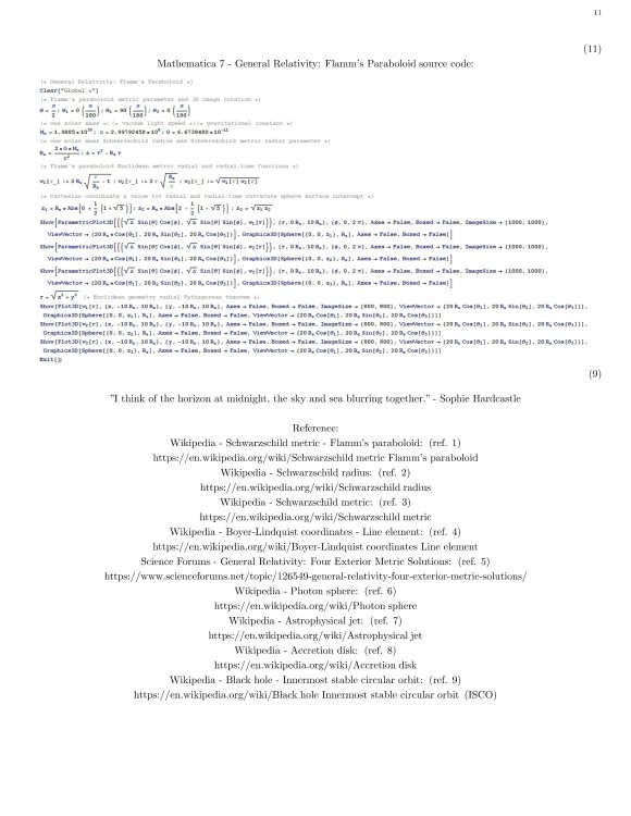
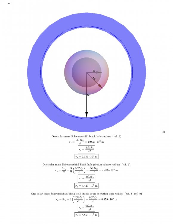
Any discussions and/or peer reviews about this specific topic thread? "I think of the horizon at midnight, the sky and sea blurring together." - Sophie Hardcastle Reference: Wikipedia - Schwarzschild metric - Flamm's paraboloid: (ref. 1) https://en.wikipedia.org/wiki/Schwarzschild_metric#Flamm's_paraboloid Wikipedia - Schwarzschild radius: (ref. 2) https://en.wikipedia.org/wiki/Schwarzschild_radius Wikipedia - Schwarzschild metric: (ref. 3) https://en.wikipedia.org/wiki/Schwarzschild_metric Wikipedia - Boyer-Lindquist coordinates - Line element: (ref. 4) https://en.wikipedia.org/wiki/Boyer-Lindquist_coordinates#Line_element Science Forums - General Relativity: Four Exterior Metric Solutions - Orion1: (ref. 5) https://www.scienceforums.net/topic/126549-general-relativity-four-exterior-metric-solutions/ Wikipedia - Photon sphere: (ref. 6) https://en.wikipedia.org/wiki/Photon_sphere Wikipedia - Astrophysical jet: (ref. 7) https://en.wikipedia.org/wiki/Astrophysical_jet Wikipedia - Accretion disk: (ref. 8) https://en.wikipedia.org/wiki/Accretion_disk Wikipedia - Black hole - Innermost stable circular orbit: (ref. 9) https://en.wikipedia.org/wiki/Black_hole#Innermost_stable_circular_orbit_(ISCO) Mathematica 7 - General Relativity - Flamm's Paraboloid source code notebook attachment: General Relativity - Flamm's Paraboloid.nb Mathematica 7 - General Relativity - Schwarzschild Black Hole Toy Model source code notebook attachment: General Relativity - Schwarzschild Black Hole Toy Model.nb Please merge the threads if there is a protocol violation.
-
Any discussions and/or peer reviews about this specific topic thread? "I think of the horizon at midnight, the sky and sea blurring together." - Sophie Hardcastle


-
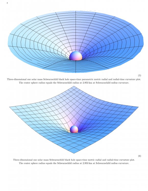
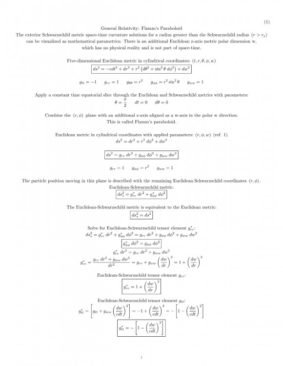
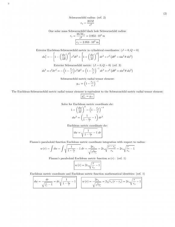
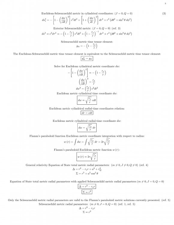
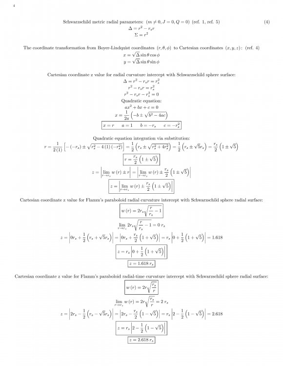
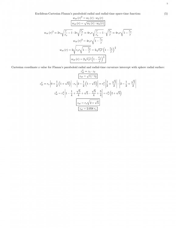
[math]\text{General Relativity: Flamm's Paraboloid}[/math] [math]\text{The exterior Schwarzschild metric space-time curvature solutions for a radius greater than the Schwarzschild radius } (r > r_{s})[/math] [math]\text{can be visualized as mathematical parametrics. There is an additional Euclidean z-axis metric polar dimension w,}[/math] [math]\text{which has no physical reality and is not part of space-time.}[/math] [math]\color{blue}{ \text{Any discussions and/or peer reviews about this specific topic thread?}}[/math] [math]\color{blue}{\text{"I think of the horizon at midnight, the sky and sea blurring together." - Sophie Hardcastle}}[/math]
-
The people who took video of police killing George Floyd and Eric Garner would have faced criminal charges in Arizona under legislation that passed approval in the Arizona state House of Representatives with only partisan support. Arizona House Bill 2319 says that "anyone who police order to stop filming" but continues to do so would "face a class 3 misdemeanor and up to 30 days in jail." (ref. 1) A 2021 ProPublica investigation found in Jefferson Parish, Louisiana, seventy-three percent (73%) of the time someone was arrested on a "cover charge" alone, they were Black Ethnicity. (ref. 2) "The 'graphic video' captured a scene drastically at odds with the initial police statement, which described the encounter as: "man dies after medical incident during police interaction." It said that George Floyd physically resisted officers and made no mention of the prolonged restraint." (ref. 3) "[Police officer], without legal justification, held Juvenile 1 by the throat and struck Juvenile 1 multiple times in the head with a flashlight. This offense included the use of a dangerous weapon, a 'flashlight' and resulted in bodily injury to Juvenile 1." - United States v. Chauvin - CASE 0:21-cr-00109-WMW-HB (2021) (ref. 4, ref. 5, ref. 6, ref. 7) "Eric Garner was killed in the New York City borough of Staten Island after [Redacted], a New York City Police Department (NYPD) officer, put him in a prohibited chokehold while arresting him. 'Video footage' of the incident generated widespread national attention and raised questions about the use of force by law enforcement." (ref. 8) Should U.S. Citizens face a class 3 misdemeanor and up to 30 days in [prison] for filming within 15 feet of police officers committing murder and/or manslaughter against another U.S. Citizen? Should U.S. Citizens face a class 3 misdemeanor and up to 30 days in [prison] for filming within 15 feet of police officers that are holding a Juvenile by the throat while striking a Juvenile multiple times in the head with a flashlight? Should U.S. Citizens face a class 3 misdemeanor and up to 30 days in [prison] for filming within 15 feet of police officers that are placing a U.S. Citizen in a prohibited chokehold while arresting them? Should U.S. Citizens be subjected to the "cover charge" of a class 3 misdemeanor and up to 30 days in [prison] for filming within 15 feet of police officers, to justify police use of excessive force, and the arrest of U.S. Citizens based upon their Black Ethnicity? Reference: House Bill 2319 - anyone who police order to stop filming but continues to do so would face a class 3 misdemeanor and up to 30 days in jail: (ref. 1) https://www.azleg.gov/legtext/55leg/2R/bills/HB2319P.pdf ProPublica - Seventy-three percent (73%) of the time someone was arrested on a "cover charge" alone, they were Black Ethnicity: (ref. 2) https://www.propublica.org/article/he-was-filming-on-his-phone-then-a-deputy-attacked-him-and-charged-him-with-resisting-arrest NPR - [Juvenile 2] who filmed George Floyds murder: (ref. 3) https://www.npr.org/sections/trial-over-killing-of-george-floyd/2021/04/21/989480867/darnella-frazier-teen-who-filmed-floyds-murder-praised-for-making-verdict-possib United States Department of Justice - United States v. Chauvin - CASE 0:21-cr-00109-WMW-HB (2021): (ref. 4) https://www.justice.gov/opa/press-release/file/1392446/download United States Department of Justice - United States v. Chauvin - CASE 0:21-cr-00108-PAM-TNL (2021): (ref. 5) https://www.justice.gov/opa/press-release/file/1392451/download United States Department of Justice - Four Police Officers Indicted on Federal Civil Rights Charges for Death of George Floyd: (ref. 6) https://www.justice.gov/opa/pr/four-former-minneapolis-police-officers-indicted-federal-civil-rights-charges-death-george Wikipedia - Murder of George Floyd: (ref. 7) https://en.wikipedia.org/wiki/Murder_of_George_Floyd Wikipedia - Killing of Eric Garner: (ref. 8) https://en.wikipedia.org/wiki/Killing_of_Eric_Garner
-
S: "It's entirely possible that the demarcation of 15' [feet] (or whatever is decided on) could be upheld. They could find that anything inside that is interference with the police." - swansont Why would a Federal Circuit Court uphold a magical fifteen foot (15') distance? What can police officers accomplish with a magical fifteen foot (15') distance, that police officers cannot accomplish with red or yellow Warning Police Tape and/or Caution Police Tape? Why would a Federal Circuit Court uphold that "anything inside [fifteen feet] would be "interference with the police."? "The Arizona Chapter of the American Civil Liberties Union disagrees." "Simply filming them [police] is not interference," said [Redacted], ACLU Arizona’s Smart Justice campaign strategist. "In terms of protecting the [police] officers, if someone is standing there holding a cell phone it does not endanger the [police] officer in any way." (ref. 1) S: "Politicians make bad laws most of the time; makes you wonder what they get paid for." - MigL In the United States, judicial review is the legal power of a court to determine if a statute, treaty, or administrative regulation contradicts or violates the provisions of existing law, a State Constitution, or ultimately the United States Constitution. (ref. 2) As of 2014, the United States Supreme Court has held 176 Acts of the U.S. Congress unconstitutional. In the period 1960–2019, the Supreme Court has held 483 laws unconstitutional in whole or in part. (ref. 2) As of 2017, the United States Supreme Court had held unconstitutional portions or the entirety of some 182 Acts of the U.S. Congress. (ref. 3) As of 2017, the United States Supreme Court had held unconstitutional portions or the entirety of some 238 State constitutional, statutory provisions and municipal ordincances. (ref. 4) As of 2018, the Supreme Court had overruled more than 300 of its own cases. (ref. 5) S: "2. it's found to be [unconstitutional] by a federal court" - swansont S: "Then if a case is brought up, the Supreme Court has to decide whether it is Constitutional." - MigL In the United States, any local, State, or Federal judge can rule any law as unconstitutional. "This [United States] Constitution, and the Laws of the United States which shall be made in Pursuance thereof; and all Treaties made, or which shall be made, under the Authority of the United States, shall be the supreme Law of the Land; and the Judges in every State shall be bound thereby, any thing in the Constitution or Laws of any State to the Contrary notwithstanding." - Article 6, Clause 2 of the United States Constitution "The Constitution of these United States is the supreme law of the land. Any law that is repugnant to the Constitution is null and void of law." "void ab initio" - Marbury v. Madison, (5 US 137) "Where Rights secured by the Constitution are involved, there can be no 'rule making' or 'legislation' which would abrogate them." - Miranda v. Arizona, (384 U.S. 426, 491; 86 S. Ct. 1603) "An unconstitutional Act is not law; it confers no Rights; it imposes no duties; affords no protection; it creates no office; it is in legal contemplation, as inoperative as though it had never been passed." - Norton v. Shelby County, (118 U.S. 425 p. 442) S: "The [partisan] has gotten a lot of judges put in place, and this is the kind of thing that chips away at [R]ights." - swansont Why would a Federal Circuit Court judge make a judicial decision based upon their partisan affiliation?, instead of by legal merit (denotes the extent to which the facts support a remedy in law) and/or by de jure "by laws" and/or de facto "in fact" case laws? S: "The political leanings of SCJ [Supreme Court Justices] play a great role in this decision, and why each [partisan] [political] party tries to fill vacancies with politically like-minded judges." - MigL [Supreme Court] Clerks hired by each of the justices of the Supreme Court are often given considerable leeway in the opinions they draft. "Supreme Court clerkship appeared to be a nonpartisan institution from the 1940s into the 1980s. (ref. 6) "As law has moved closer to mere politics, political affiliations have naturally and predictably become proxies for the different political agendas that have been pressed in and through the courts"; the [Supreme] Court had thus begun to mirror the political branches of government; This politicized hiring trend reinforces the impression that the Supreme Court is "a super-legislature responding to ideological arguments rather than a legal institution responding to concerns grounded in the rule of law." (ref. 6) A poll conducted in June 2012 by The New York Times and CBS News showed just [forty-four percent] (44%) of Americans [U.S. Citizens] approve of the job the Supreme Court is doing. Three-quarters [seventy-five percent] (75%) said justices' decisions are sometimes influenced by their political or personal views. (ref. 6) Reference: Arizona Mirror - Ex Cop Lawmaker Wants To Restrict Recording Videos Of Cops: (ref. 1) https://www.azmirror.com/blog/ex-cop-lawmaker-wants-to-restrict-recording-videos-of-cops/ Wikipedia - Judicial review in the United States: (ref. 2) https://en.wikipedia.org/wiki/Judicial_review_in_the_United_States Wikipedia - Judicial review in the United States: (ref. 3) https://en.wikipedia.org/wiki/Judicial_review_in_the_United_States#Judicial_review_after_Marbury GovInfo - State Constitutional And Statutory Provisions And Municipal Ordincances Held Unconstitutional (ref. 4) https://www.govinfo.gov/content/pkg/GPO-CONAN-2017/pdf/GPO-CONAN-2017-12.pdf Wikipedia - List of overruled United States Supreme Court decisions: (ref. 5) https://en.wikipedia.org/wiki/List_of_overruled_United_States_Supreme_Court_decisions Wikipedia - Supreme Court of the United States - Politicization of the Court: (ref. 6) https://en.wikipedia.org/wiki/Supreme_Court_of_the_United_States#Politicization_of_the_Court
-
S: "unconstitutional" "is what the supreme court says it is, though this would probably get struck down in whatever federal district it's in first. But it will likely take a while for that to happen." - swansont Q: "Why is Ben Franklin's name redacted?" - swansont So that he would not be subjected to unconstitutional prior restraint penalties and deprivation of liberty for the exercise of free speech. The unconstitutional bill now goes to the Arizona Senate for a divided partisan vote. The Arizona Senate has a divided partisan ratio of 16-14. (ref. 1) The bill passed out of the Arizona House of Representatives on a 31-28 vote. In Arizona, each bill normally needs a simple majority vote to pass it out of the body (16 votes in the Senate, 31 in the House). Ninth Circuit (with jurisdiction over Alaska, Arizona, California, Guam, Hawaii, Idaho, Montana, Nevada, the Northern Mariana Islands, Oregon, and Washington). The United States Federal Ninth Circuit Court: "material fact exists concerning whether [Police] interfered with Fordyce's First Amendment Right to gather news." - Fordyce v. City of Seattle, 55 F.3d 436, 438 (9th Cir. 1995) (ref. 2) "Defendants [police officers] stopped Plaintiff only to get him to delete the pictures from his cell phone, and then arrested him only because of his repeated challenges to their authority. Such circumstances would make Plaintiff’s arrest an illegal retaliatory arrest and prior restraint." - Adkins v. Limtiaco, No. 11-17543, 2013 WL 4046720 (9th Cir. Aug. 12, 2013) (ref. 3) "there is a constitutional Right of the public to film the official activities of police officers in a public place." - Hawaii v. Russo (2017) - Supreme Court of Hawaii. (ref. 4) Q: "I think the prior restraint issue will torpedo this legislation in federal court. What do YOU think , @Orion? In your own words?" - TheVat Arizona House Bill 2319 states that "anyone who police order to stop filming" but continues to do so would "face a class 3 misdemeanor and up to 30 days in jail." Arizona House Bill 2319 is specifically enforcing unconstitutional prior restraint penalties for the First Amendment exercise of free speech, journalism and press prior to publication. (ref. 5) A prior restraint is an official government restriction of free speech, journalism and press prior to publication. Prior restraints are viewed by the United States Supreme Court as "the most serious and the least tolerable infringement on First Amendment Rights" - Nebraska Press Association v. Stuart, 427 U.S. 539 (1976) (ref. 5, ref. 6) If passed, Arizona House Bill 2319 is expected to be struck down as "unconstitutional" in the United States Federal Ninth Circuit Court within 3 years. Reference: Wikipedia - Arizona Senate - Current Members 2021-2023: (ref. 1) https://en.wikipedia.org/wiki/Arizona_Senate#Current_Members,_2021–2023 Fordyce v. City of Seattle, 55 F.3d 436, 438 (9th Cir. 1995): (ref. 2) https://caselaw.findlaw.com/us-9th-circuit/1054985.html Adkins v. Limtiaco, No. 11-17543, 2013 WL 4046720 (9th Cir. Aug. 12, 2013): (ref. 3) https://www.govinfo.gov/content/pkg/USCOURTS-gud-1_09-cv-00029/pdf/USCOURTS-gud-1_09-cv-00029-2.pdf Hawaii v. Russo (2017) - Supreme Court of Hawaii: (ref. 4) https://cases.justia.com/hawaii/supreme-court/2017-scwc-14-0000986-0.pdf Nebraska Press Association v. Stuart, 427 U.S. 539 (1976) - United States Supreme Court (ref. 5) https://tile.loc.gov/storage-services/service/ll/usrep/usrep427/usrep427539/usrep427539.pdf Wikipedia - Prior restraint: (ref. 6) https://en.wikipedia.org/wiki/Prior_restraint
-
Q: "What event(s) initiated the apparent need for that legislation?" - StringJunky "[Partisan] said he initially got the idea to run the bill because he had "seen stories" of "groups of people" going around "filming police". (ref. 1) It is not clarified in the news reports as to what "groups of people" this partisan is referring to. Perhaps this partisan is referring to "We The People". "The Arizona Chapter of the American Civil Liberties Union disagrees." "Simply filming them [police] is not interference," said [Redacted], ACLU Arizona’s Smart Justice campaign strategist. "In terms of protecting the [police] officers, if someone is standing there holding a cell phone it does not endanger the [police] officer in any way." (ref. 1) Q: "When did [Redacted] become their Governor?" - J.C.MacSwell "Whoever would overthrow the liberty of a nation, would first subdue free speech." - [Redacted] The prior restraint draconian judicial suppression of material that would be published or broadcast of free speech, journalism, and free press is the first agenda item that totalitarian and authoritarian dictators engage in either to ascend to, or maintain non-authentic draconian, totalitarian and authoritarian political pseudo-power. History indicates that such prior restraint draconian judicial suppression and totalitarian desperation extracts a heavy expenditure upon humanity. The Russian government has deployed draconian laws and outlawed and criminalized all forms of free speech, journalism and free press in Russia. It is one of the only non-authentic draconian means by which totalitarian authoritarian dictators can maintain political pseudo-power, through a censorship propaganda war against their own people. Russia increases censorship with new law: prior restraint 15 years in [prison] for free speech and press. (ref. 2) A prior restraint is an official government restriction of free speech, journalism and press prior to publication. Prior restraints are viewed by the United States Supreme Court as "the most serious and the least tolerable infringement on First Amendment Rights" - Nebraska Press Association v. Stuart, 427 U.S. 539 (1976) (ref. 3) Reference: Arizona Mirror - Ex Cop Lawmaker Wants To Restrict Recording Videos Of Cops: (ref. 1) https://www.azmirror.com/blog/ex-cop-lawmaker-wants-to-restrict-recording-videos-of-cops/ USA Today - Russia increases censorship with new law: prior restraint 15 years in [prison] for free speech and press: (ref. 2) https://www.usatoday.com/story/news/world/ukraine/2022/03/08/russia-free-speech-press-criminalization-misinformation/9433112002/ Wikipedia - Prior restraint: (ref. 3) https://en.wikipedia.org/wiki/Prior_restraint
-
Arizona House Legislature Passes Unconstitutional Bill... Arizona House Legislature approve bill to restrict "who can film police officers" and "when and where." (ref. 1) The people who took video of police killing George Floyd and Eric Garner would have faced criminal charges in Arizona under legislation that passed approval in the Arizona state House of Representatives with only partisan support. A bill proposed would make it "unlawful for someone to film police from up to 15 feet away" while officers are engaged in "law enforcement activity." Constitutional experts and Civil Rights advocates say the proposed law would be blatantly unconstitutional. Arizona House Bill 2319 says that "anyone who police order to stop filming" but continues to do so would "face a class 3 misdemeanor and up to 30 days in jail." The bill passed out of the Arizona House of Representatives on a 31-28 vote, with partisan legislature supporting it and other partisan legislature in opposition. An amendment added by the House Appropriations Committee "allows people to film their own interactions with police", as long as they are "not interfering with lawful police actions, including searching handcuffing or administering a field sobriety test." The amendment also "allows passengers in a vehicle to film" as long as they do not "interfere" with "lawful police actions." The amendment also "limits what could not be filmed from closer than 15 feet": questioning a "suspicious person", conducting an arrest, issuing a "summons" or "enforcing the law," and handling an "emotionally disturbed" or "disorderly person" who is exhibiting "abnormal behavior". Filming of police has played an integral role in helping journalists and researchers learn the breadth of how law enforcement use "cover charges" to justify the use of excessive force. The term is often used by defense attorneys to describe the charges used by police to cover up bad behavior or explain away the use of excessive force. In Chicago, it was found that two out of every three times the Chicago Police Department used force since 2004, they arrested the person on one of these types of charges. And a 2021 ProPublica investigation found in Jefferson Parish, Louisiana, seventy-three percent (73%) of the time someone was arrested on a "cover charge" alone, they were Black Ethnicity. (ref. 2) The unconstitutional bill now goes to the Arizona Senate for a divided partisan vote. --- A Federalist Paper: Credo id quoda video. "I believe that what we see." A Constitutionalist Response: The Supremacy Clause is the provision in Article 6, Clause 2 of the United States Constitution that establishes the Constitution, AS THE SUPREME LAW OF THE LAND. No state can make a higher law and if it tried no judge could enforce any such law. That law would become a legal fiction, as if it never existed. "The Constitution of these United States is the supreme law of the land. Any law that is repugnant to the Constitution is null and void of law." "void ab initio" - Marbury v. Madison, (5 US 137) "Where Rights secured by the Constitution are involved, there can be no 'rule making' or legislation which would abrogate them." - Miranda v. Arizona, (384 U.S. 426, 491; 86 S. Ct. 1603) "An unconstitutional act is not law; it confers no Rights; it imposes no duties; affords no protection; it creates no office; it is in legal contemplation, as inoperative as though it had never been passed." - Norton v. Shelby County, (118 U.S. 425 p. 442) The Supreme Court declined to establish that the "press" had Rights which the average citizen did not. ALL U.S. citizens have the same Right of access to information that the "press" has. - Smith v. City of Cumming 212 F.3d 1332 (11th Cir. 2000), Branzburg v. Hayes, 408 U.S. 665 (1972), New York Times Co. v. Sullivan, 376 U.S. 254 (1964) A prior restraint is an official government restriction of free speech, journalism and press prior to publication. Prior restraints are viewed by the United States Supreme Court as "the most serious and the least tolerable infringement on First Amendment Rights" - Nebraska Press Association v. Stuart, 427 U.S. 539 (1976) (ref. 4) "No state legislator or executive or judicial officer can war against the Constitution without violating his undertaking [Oath] to support it." - Cooper v. Aaron, 358 U.S. 1, 78 S.Ct. 1401 (1958) "The claim and exercise of a Constitutional Right cannot be converted into a crime"... "a denial of them would be a denial of due process of law." - Wright v. Georgia, 373 U.S. 284 (1963), Simmons v. United States, 390 U.S. 377 (1968), Palmer v. City of Euclid, 402 U.S. 544 (1971), Sherar v. Cullen, 481 F.2d 945 (9th Cir. 1973) "No state shall convert a liberty into a privilege, license it, and attach a fee to it." - Murdock v. Pennsylvania, (319 US 105) "If the state converts a liberty into a privilege, the citizen can engage in the Right with impunity." - Shuttlesworth v. Birmingham, 373 US 262 "Changes in technology and society have made the lines between private citizen and journalist exceedingly difficult to draw. The proliferation of electronic devices with video-recording capability means that many of our images of current events come from bystanders with a ready cell phone or digital camera rather than a traditional film crew, and news stories are now just as likely to be broken by a blogger at their computer as a reporter at a major newspaper. Such developments make clear why the news-gathering protections of the First Amendment cannot turn on professional credentials or status." - Glik v. Cunniffe, 655 F. 3d 78 - Court of Appeals, (1st Cir. 2011) The majority Federal Electoral College districts within the United States Federal Circuit Courts have ruled that there is a First Amendment Right to record police activity in public. Turner v. Driver, No. 16-10312 (5th Cir. 2017), Fields v. City of Philadelphia, No. 16-1650 (3d Cir. 2017), Garcia v. Montgomery Cty., Maryland, 145 F. Supp. 3d 492, 508 (4th Cir. 2015), Ramos v. Flowers, Docket No. A-4910-10T3 (N.J. App. Div. Sept. 21, 2012), ACLU v. Alvarez, 679 F.3d 583, 595 (7th Cir. 2012), Glik v. Cunniffe, 655 F. 3d 78 - Court of Appeals, (1st Cir. 2011), Smith v. City of Cumming, 212 F.3d 1332, 1333 (11th Cir. 2000), Robinson v. Fetterman, 378 F. Supp. 2d 534 (3rd Cir. 2005), Fordyce v. City of Seattle, 55 F.3d 436, 438 (9th Cir. 1995) First Circuit (with jurisdiction over Maine, Massachusetts, New Hampshire, Puerto Rico, and Rhode Island): see Glik v. Cunniffe, 655 F.3d 78, 85 (1st Cir. 2011) ("[A] citizen's Right to film government officials, including law enforcement officers, in the discharge of their duties in a public space is a basic, vital, and well-established liberty safeguarded by the First Amendment."); Iacobucci v. Boulter, 193 F.3d 14 (1st Cir. 1999) (police lacked authority to prohibit citizen from recording commissioners in town hall "because [the citizen's] activities were peaceful, not performed in derogation of any law, and done in the exercise of his First Amendment Rights[.]"). Gericke v. Begin, 753 F.3d 1 (1st Cir. 2014) ("[a] traffic stop, no matter the additional circumstances, is inescapably a police duty carried out in public. Hence, a traffic stop does not extinguish an individual’s Right to film.") Third Circuit (with jurisdiction over Delaware, New Jersey, Pennsylvania): see Robinson v. Fetterman, 378 F. Supp. 2d 534 (E.D. Pa. 2005) ("As we explained above, the activity of Robinson in videotaping the defendants on October 23, 2002, was constitutionally protected speech. Robinson was filming the troopers while on private property with authorization from the landowner. He was 20 to 30 feet from them and at no time did he interfere with the carrying out of the troopers' duties, which were being conducted on or near a public highway.") Gilles v. Davis, 427 F.3d 197, 212 n.14 (3d Cir. 2005) ("videotaping or photographing the police in the performance of their duties on public property may be a protected activity.") "it is indisputable that all officers in the Philadelphia Police Department were put on actual notice that they were required to uphold the First Amendment Right to make recordings of police activity. From a practical perspective, the police officers had no ground to claim ambiguity about the boundaries of the citizens’ constitutional Right here." - Fields v. City of Philadelphia, No. 16-1650 (3d Cir. 2017) Fourth Circuit (with jurisdiction over Maryland, North Carolina, Virginia, West Virginia): see Garcia v. Montgomery Cty., Maryland, 145 F. Supp. 3d 492, 508 (D. Maryland Nov. 2, 2015) (The "Right to record public police activities... if done peacefully and without interfering with the performance of police duties, is protected by the First Amendment.") Fifth Circuit (with jurisdiction over Louisiana, Mississippi, Texas): see Turner v. Driver, No. 16-10312 (5th Cir. 2017) ("a First Amendment Right to record the police does exist, subject only to reasonable time, place, and manner restrictions.” The majority derives this general Right to film the police from “First Amendment principles, controlling authority, and persuasive precedent.") Seventh Circuit (with jurisdiction over Illinois, Indiana, and Wisconsin): see ACLU v. Alvarez, 679 F.3d 583, 595 (7th Cir. 2012) ("The act of making an audio or audiovisual recording is necessarily included within the First Amendment's guarantee of speech and press Rights as a corollary of the Right to disseminate the resulting recording."). Ninth Circuit (with jurisdiction over Alaska, Arizona, California, Guam, Hawaii, Idaho, Montana, Nevada, the Northern Mariana Islands, Oregon, and Washington): see Fordyce v. City of Seattle, 55 F.3d 436, 438 (9th Cir. 1995) (assuming a First Amendment Right to record the police); see also Adkins v. Limtiaco, No. 11-17543, 2013 WL 4046720 (9th Cir. Aug. 12, 2013) (recognizing First Amendment Right to photograph police, citing Fordyce). Hawaii v. Russo (2017) ("there is a constitutional Right of the public to film the official activities of police officers in a public place.") Eleventh Circuit (with jurisdiction over Alabama, Florida and Georgia): see Smith v. City of Cumming, 212 F.3d 1332, 1333 (11th Cir. 2000) ("The First Amendment protects the Right to gather information about what public officials do on public property, and specifically, a Right to record matters of public interest."). The Appellate Division of the Superior Court of New Jersey likewise recognized the existence of such a Right in Ramos v. Flowers, Docket No. A-4910-10T3 (N.J. App. Div. Sept. 21, 2012), relying heavily on the First Circuit's reasoning in the Glik v. Cunniffe, (2011), case law. The United States Department of Justice, Civil Rights Division, issued recommendations on May 14th, 2012, (DJ 207-35-10 section 2 A), that all police departments "affirmatively set forth the First Amendment Right to record police activity." The United States Department of Justice has openly stated its position that the First Amendment protects all U.S. citizens who record the activities of the police in public, and has intervened in at least one Civil Rights lawsuit against police officers to support that First Amendment Right. See Sharp v. Baltimore City Police Dep't, No. 1:11-cv-02888-BEL (D. Md. Statement of Interest filed January 10, 2012) "Constitutional Rights would be of little value if they could be indirectly denied." - Gomillion v. Lightfoot, 364 U.S. 155 (1966), Smith v. Allwright, 321 U.S. 649.644, (1944) "There can be no sanction or penalty imposed upon one because of his exercise of Constitutional Rights." - Sherar v. Cullen, 481 F. 2d 946 (1973) "Where an individual is detained, without a warrant and without having committed a crime (filming police in public is a constitutionally protected activity and is not a crime), the detention is a false arrest and false imprisonment." Damages Awarded: Trezevant v. City of Tampa, 241 F2d. 336 (11th Cir 1984) "[Police] officers of the court have no [Qualified] immunity, when violating a Constitutional Right, from liability. For they are deemed to know the law!" - Owen v. Independence, 100 S.C.T. 1398, 445 US 622, Williamson v. Mills, 11th Cir., 1995, Brookfield Construction Co. v. Stewart, (1964) "Qualified immunity defense fails if the public [police] officer violates clearly established Rights, because a reasonably competent official should know the law governing his conduct." - Jones v. Counce, 7-F3d-1359-8th Cir (1993), Benitez v. Wolff, 985-F3d 662 2nd Cir (1993) When an illegal arrest is made the [police] officers involved waive their [Qualified] immunity and are liable for damages done to the one arrested. (Title 18 Code 1911) - violations of oath of office. Quern vs. Jordan 440, U.S. 332, 345 (1979) If two or more persons conspire to injure, oppress, threaten, or intimidate any person in any State, Territory, Commonwealth, Possession, or District in the free exercise or enjoyment of any Right or privilege secured to him by the Constitution or laws of the United States, they shall be fined under this title or imprisoned for any term of years or for life, or both, or may be sentenced to death. (18 U.S. Code § 241 - Conspiracy against Constitutional Rights) Whoever, under color of any law, statute, ordinance, regulation, or custom, willfully subjects any person in any State, Territory, Commonwealth, Possession, or District to the deprivation of any Rights, privileges, or immunities secured or protected by the Constitution or laws of the United States, shall be fined under this title or imprisoned not more than one year, or both. (18 U.S. Code § 242 - Deprivation of Rights under color of law) Every person who, under color of any statute, ordinance, regulation, custom, or usage, of any State or Territory or the District of Columbia, subjects, or causes to be subjected, any citizen of the United States or other person within the jurisdiction thereof to the deprivation of any Rights, privileges, or immunities secured by the Constitution and laws, shall be liable to the party injured in an action at law, suit in equity, or other proper proceeding for redress. (42 U.S. Code § 1983 - Civil action for deprivation of Rights) A journalist is defined as "Someone who engages in journalism." - Merriam-Webster Dictionary (2022) Journalism is defined as "The collection and editing of news for presentation through writing or the media; the public press." - Merriam-Webster Dictionary (2022) "The people shall not be deprived or abridged of their Right to speak, to write, or to publish their sentiments; and the freedom of the press, as one of the great bulwarks of liberty, shall be inviolable." - James Madison "Our liberty depends on the freedom of the press, and that cannot be limited without being lost." - Thomas Jefferson (1786) "Whoever would overthrow the liberty of a nation, would first subdue free speech." - Benjamin Franklin In November 2018, the Bureau of Justice Statistics published a report on the use of body-worn cameras by law enforcement agencies in the United States in 2016: Only forty-seven percent (47%) of general-purpose law enforcement agencies had acquired body-worn cameras, and for large police departments, that number is only eighty percent (80%). (ref. 3) "The record in this case includes a 'videotape' capturing the events in question." "...the 'record' blatantly contradicts the [subject's] version of events so that no reasonable jury could believe it, a court should not adopt that version of the facts for purposes of ruling on a summary judgment motion." - United States Supreme Court - Scott v. Harris, 550 U.S. 372 (2007) Credo id quoda video. "I believe that what we see." Any discussions and/or peer reviews about this specific topic thread? Reference: House Bill 2319 - anyone who police order to stop filming but continues to do so would face a class 3 misdemeanor and up to 30 days in jail: (ref. 1) https://www.azleg.gov/legtext/55leg/2R/bills/HB2319P.pdf Arizona Mirror - House Republicans approve bill to restrict who can film cops and when and where: (ref. 2) https://www.azmirror.com/2022/02/23/house-republicans-approve-bill-to-restrict-who-can-film-cops-and-when/ United States National Institute For Justice - Research on Body-Worn Cameras and Law Enforcement: (ref. 3) https://nij.ojp.gov/topics/articles/research-body-worn-cameras-and-law-enforcement Wikipedia - Prior restraint: (ref. 4) https://en.wikipedia.org/wiki/Prior_restraint
-
[math]\color{blue}{\text{Page 1 updated with more detailed steps...}}[/math] [math]\;[/math] [math]\color{blue}{\text{What distinguishes this theoretical approach from mainstream science?}}[/math] [math]\;[/math] [math]\color{blue}{\text{Any discussions and/or peer reviews about this specific topic thread?}}[/math] [math]\;[/math]
-
-
[math]\boxed{\color{blue}{\bigotimes} \; \int f(\color{blue}{n}) \; \text{SCIENCE} \color{blue}{\text{FORUMS}} \text{.NET}}[/math]

-
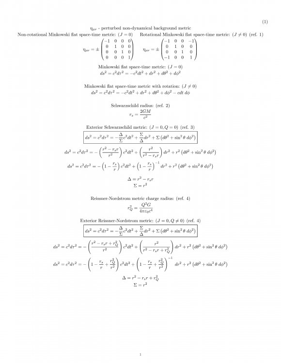
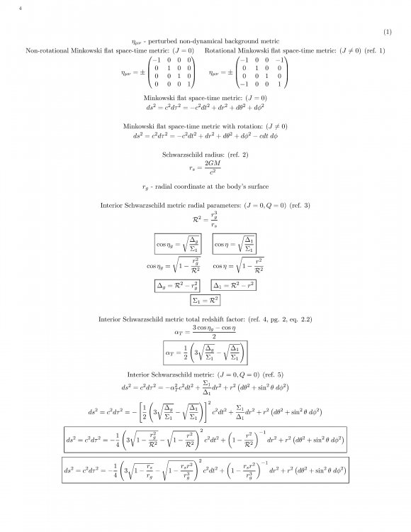
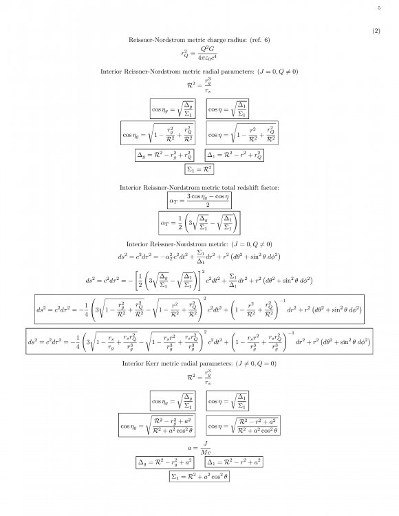
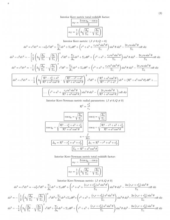
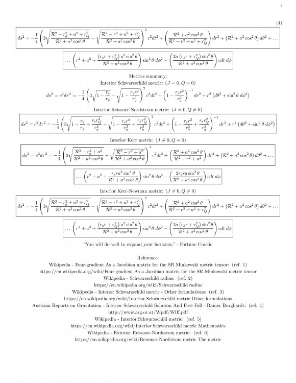
In Einstein's theory of general relativity, the interior metric or interior fluid solution, is an exact solution to the Einstein field equations and Einstein-Maxwell equations that describes the gravitational field and the space-time geometry in the interior of a non-rotating or rotating neutral or charged spherically symmetric body of mass M, which consists of an incompressible fluid and constant density throughout the body and has zero pressure at the surface and that the electric charge and angular momentum of the mass may be zero or non-zero, and the universal cosmological constant is zero. For a non-zero charged mass, the metric takes into account the Einstein-Maxwell field energy of an electromagnetic field within the space-time geometry. The space-time geometry is in Boyer-Lindquist coordinates. "yet still idealized family of solutions would be the Vaidya spacetimes." - Markus Hanke Are these Vaidya metrics mathematically mapped out accurately at this point? "Mass, charge and spin are global properties of the entire spacetime - you cannot localise these quantities at any particular place." - Markus Hanke What if the black hole quantum charge originates from its center core? "We analyze the “vacuum” polarization induced by a quantum charged scalar field near the inner horizon of a charged black hole in quantum states evolving from arbitrary regular in states." "As the formation of charged BHs necessitates the presence of charged matter, it is actually more natural to consider a charged scalar field" "At the event horizon HR, this current is responsible for the discharge of the BH via Hawking radiation." (ref .7) The model in reference 7, appears to be modeling the field interaction between a black hole that is quantum charged at its core, and with the charged matter near the inner horizon, which discharges as hawking radiation. What determines the charge magnitude and polarity of a quantum charged black hole? The black hole core quantum charge cannot extend past the inner event horizon? Any discussions and/or peer reviews about this specific topic thread? "You will do well to expand your horizons." - Fortune Cookie Reference: Wikipedia - Four-gradient As a Jacobian matrix for the SR Minkowski metric tensor: (ref. 1) https://en.wikipedia.org/wiki/Four-gradient#As_a_Jacobian_matrix_for_the_SR_Minkowski_metric_tensor Wikipedia - Schwarzschild radius: (ref. 2) https://en.wikipedia.org/wiki/Schwarzschild_radius Wikipedia - Interior Schwarzschild metric - Other formulations: (ref. 3) https://en.wikipedia.org/wiki/Interior_Schwarzschild_metric#Other_formulations Austrian Reports on Gravitation - Interior Schwarzschild Solution And Free Fall - Rainer Burghardt: (ref. 4) http://www.arg.or.at/Wpdf/WIff.pdf Wikipedia - Interior Schwarzschild metric: (ref. 5) https://en.wikipedia.org/wiki/Interior_Schwarzschild_metric#Mathematics Wikipedia - Exterior Reissner-Nordstrom metric: (ref. 6) https://en.wikipedia.org/wiki/Reissner–Nordström_metric#The_metric Quantum (dis)charge of black hole interiors - Christiane Klein: (ref. 7) https://arxiv.org/pdf/2103.03714.pdf Wikipedia - Vaidya metric: (ref. 8) https://en.wikipedia.org/wiki/Vaidya_metric

.thumb.jpg.600e6db1f2e8ca1da8d5eaa84b55baf8.jpg)
-
In Einstein's theory of general relativity, the interior metric or interior fluid solution, is an exact solution to the Einstein field equations and Einstein-Maxwell equations that describes the gravitational field and the space-time geometry in the interior of a non-rotating or rotating neutral or charged spherically symmetric body of mass M, which consists of an incompressible fluid and constant density throughout the body and has zero pressure at the surface and that the electric charge and angular momentum of the mass may be zero or non-zero, and the universal cosmological constant is zero. For a non-zero charged mass, the metric takes into account the Einstein-Maxwell field energy of an electromagnetic field within the space-time geometry. The space-time geometry is in Boyer-Lindquist coordinates. [math]\color{blue}{\text{Any discussions and/or peer reviews about this specific topic thread?}}[/math] [math]\;[/math] [math]\color{blue}{\text{"You will do well to expand your horizons." - Fortune Cookie}}[/math] [math]\;[/math] Reference: Wikipedia - Four-gradient As a Jacobian matrix for the SR Minkowski metric tensor: (ref. 1) https://en.wikipedia.org/wiki/Four-gradient#As_a_Jacobian_matrix_for_the_SR_Minkowski_metric_tensor Wikipedia - Schwarzschild radius: (ref. 2) https://en.wikipedia.org/wiki/Schwarzschild_radius Wikipedia - Interior Schwarzschild metric - Other formulations: (ref. 3) https://en.wikipedia.org/wiki/Interior_Schwarzschild_metric#Other_formulations Austrian Reports on Gravitation - Interior Schwarzschild Solution And Free Fall - Rainer Burghardt: (ref. 4) http://www.arg.or.at/Wpdf/WIff.pdf Wikipedia - Interior Schwarzschild metric: (ref. 5) https://en.wikipedia.org/wiki/Interior_Schwarzschild_metric#Mathematics Wikipedia - Exterior Reissner-Nordstrom metric: (ref. 6) https://en.wikipedia.org/wiki/Reissner–Nordström_metric#The_metric


-
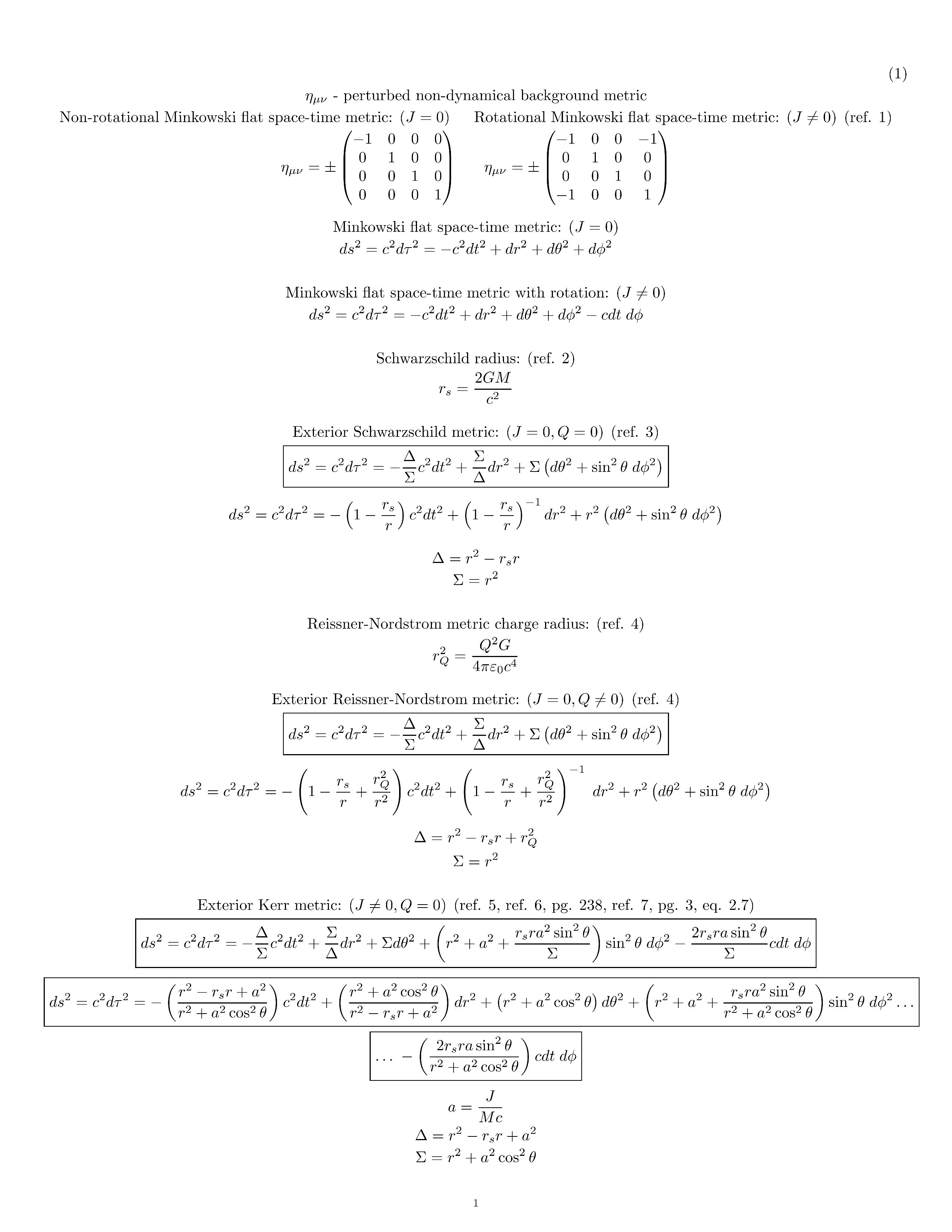
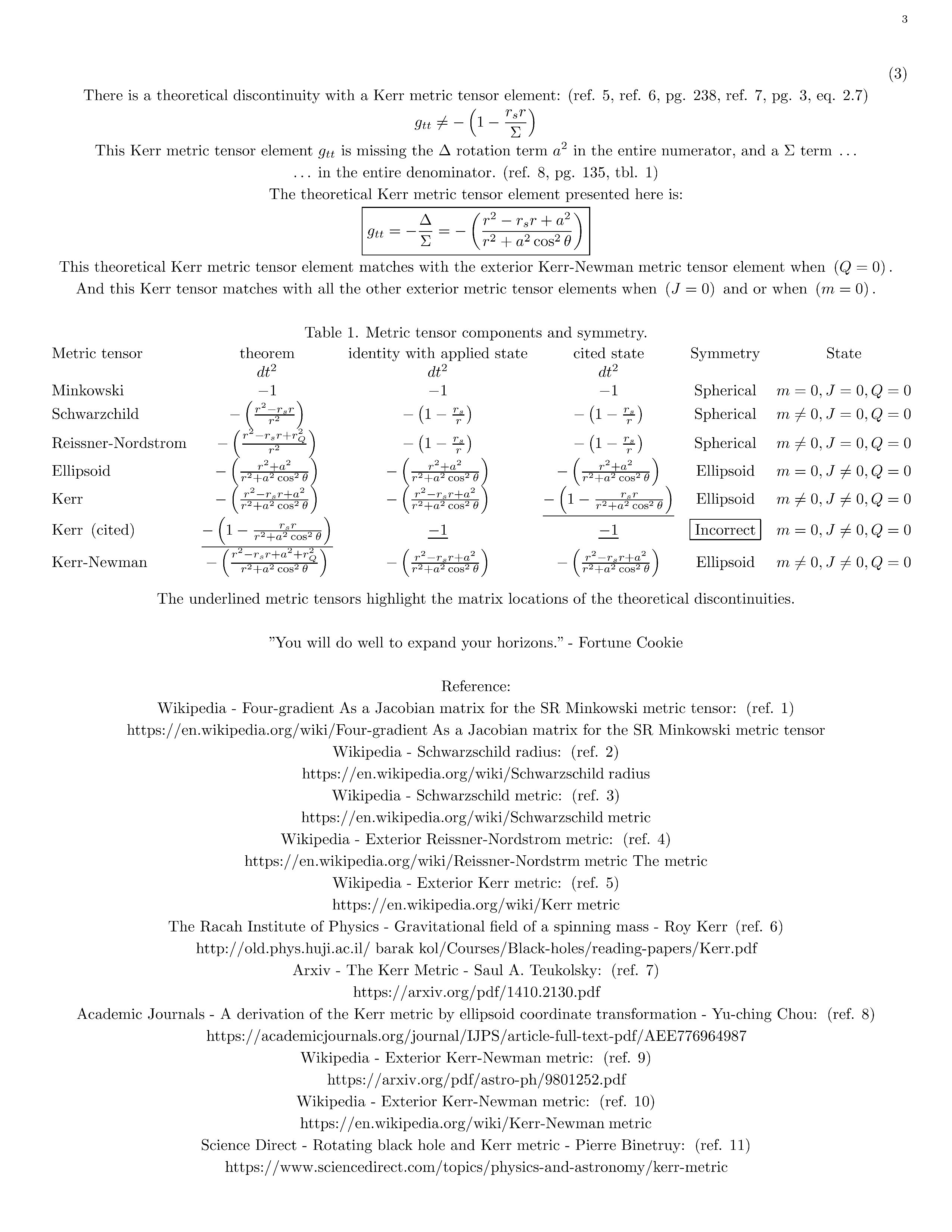
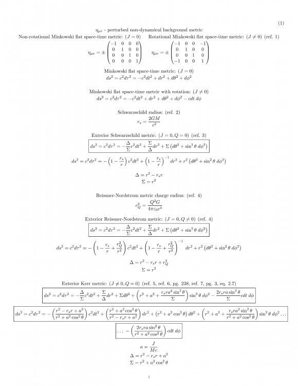
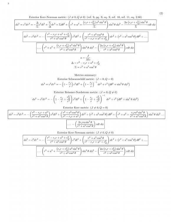
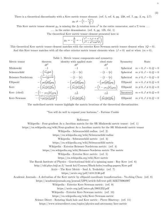
In Einstein's theory of general relativity, the exterior metric or exterior fluid solution, is an exact solution to the Einstein field equations and Einstein-Maxwell equations that describes the gravitational field and the space-time geometry in the exterior of a non-rotating or rotating neutral or charged spherically symmetric body of mass M, which consists of an incompressible fluid and constant density throughout the body and has zero pressure at the surface and that the electric charge and angular momentum of the mass may be zero or non-zero, and the universal cosmological constant is zero. For a non-zero charged mass, the metric takes into account the Einstein-Maxwell field energy of an electromagnetic field within the space-time geometry. The space-time geometry is in Boyer-Lindquist coordinates. There is a theoretical discontinuity with a Kerr metric tensor element: (ref. 5, ref. 6, pg. 238, ref. 7, pg. 3, eq. 2.7) [math]g_{tt} \neq -\left(1 - \frac{r_{s} r}{\Sigma} \right)[/math] This Kerr metric tensor element [math]g_{tt}[/math] is missing the [math]\Delta [/math] rotation term [math]a^{2}[/math] in the entire numerator, and a [math]\Sigma[/math] term in the entire denominator. (ref. 8` pg. 135` tbl. 1) [math]\color{blue}{\text{The theoretical Kerr metric tensor element presented here is:}}[/math] [math]\boxed{g_{tt} = -\frac{\Delta}{\Sigma} = -\left(\frac{r^{2} - r_{s} r + a^{2}}{r^{2} + a^{2} \cos^{2} \theta} \right)}[/math] [math]\color{blue}{\text{This theoretical Kerr metric tensor element matches with the exterior Kerr-Newman metric tensor element when } (Q = 0) \text{.}}[/math] [math]\color{blue}{\text{And this Kerr tensor matches with all the other exterior metric tensor elements when } (J = 0) \text{ and or when } (m = 0) \text{.}}[/math] [math]\;[/math] [math]\color{blue}{\text{Table 1. Metric tensor components and symmetry.}}[/math] [math]\begin{array}{l*{5}c} \text{Metric tensor} & \text{theorem} & \text{identity with applied state} & \text{cited state} & \text{Symmetry} & \text{State} \\ \text{} & dt^{2} & dt^{2} & dt^{2} & \text{} \\ \text{Minkowski} & -1 & -1 & -1 & \text{Spherical} & m = 0,J = 0,Q = 0 \\ \text{Schwarzchild} & -\left(\frac{r^{2} - r_{s} r}{r^{2}} \right) & -\left(1 - \frac{r_{s}}{r} \right) & -\left(1 - \frac{r_{s}}{r} \right) & \text{Spherical} & m \neq 0,J = 0,Q = 0 \\ \text{Reissner-Nordstrom} & -\left(\frac{r^{2} - r_{s} r + r_{Q}^{2}}{r^{2}} \right) & -\left(1 - \frac{r_{s}}{r} \right) & -\left(1 - \frac{r_{s}}{r} \right) & \text{Spherical} & m \neq 0,J = 0,Q = 0 \\ \text{Ellipsoid} & -\left(\frac{r^{2} + a^{2}}{r^{2} + a^{2} \cos^{2} \theta} \right) & -\left(\frac{r^{2} + a^{2}}{r^{2} + a^{2} \cos^{2} \theta} \right) & -\left(\frac{r^{2} + a^{2}}{r^{2} + a^{2} \cos^{2} \theta} \right) & \text{Ellipsoid} & m = 0,J \neq 0,Q = 0 \\ \text{Kerr} & -\left({\frac{r^{2} - r_{s}r + a^{2}}{r^{2} + a^{2} \cos^{2} \theta}} \right) & -\left({\frac{r^{2} - r_{s}r + a^{2}}{r^{2} + a^{2} \cos^{2} \theta}} \right) & \underline{-\left(1 - \frac{r_{s} r}{r^{2} + a^{2} \cos^{2} \theta} \right)} & \text{Ellipsoid} & m \neq 0,J \neq 0,Q = 0 \\ \text{Kerr } \left(\text{cited} \right) & \underline{-\left(1 - \frac{r_{s} r}{r^{2} + a^{2} \cos^{2} \theta} \right)} & \underline{-1} & \underline{-1} & \boxed{\text{Incorrect}} & m = 0,J \neq 0,Q = 0 \\ \text{Kerr-Newman} & -\left(\frac{r^{2} - r_{s} r + a^{2} + r_{Q}^{2}}{r^{2} + a^{2} \cos^{2} \theta} \right) & -\left(\frac{r^{2} - r_{s} r + a^{2}}{r^{2} + a^{2} \cos^{2} \theta} \right) & -\left(\frac{r^{2} - r_{s} r + a^{2}}{r^{2} + a^{2} \cos^{2} \theta} \right) & \text{Ellipsoid} & m \neq 0, J \neq 0, Q = 0 \\ \end{array}[/math] [math]\;[/math] [math]\color{blue}{\text{The underlined metric tensors highlight the matrix locations of the theoretical discontinuities.}}[/math] [math]\;[/math] [math]\color{blue}{\text{Any discussions and/or peer reviews about this specific topic thread?}}[/math] [math]\;[/math] [math]\color{blue}{\text{"You will do well to expand your horizons." - Fortune Cookie}}[/math] [math]\;[/math] Reference: Wikipedia - Four-gradient As a Jacobian matrix for the SR Minkowski metric tensor: (ref. 1) https://en.wikipedia.org/wiki/Four-gradient#As_a_Jacobian_matrix_for_the_SR_Minkowski_metric_tensor Wikipedia - Schwarzschild radius: (ref. 2) https://en.wikipedia.org/wiki/Schwarzschild_radius Wikipedia - Schwarzschild metric: (ref. 3) https://en.wikipedia.org/wiki/Schwarzschild_metric Wikipedia - Exterior Reissner-Nordstrom metric: (ref. 4) https://en.wikipedia.org/wiki/Reissner–Nordström_metric#The_metric Wikipedia - Exterior Kerr metric: (ref. 5) https://en.wikipedia.org/wiki/Kerr_metric The Racah Institute of Physics - Gravitational field of a spinning mass - Roy Kerr (ref. 6) http://old.phys.huji.ac.il/~barak_kol/Courses/Black-holes/reading-papers/Kerr.pdf Arxiv - The Kerr Metric - Saul A. Teukolsky: (ref. 7) https://arxiv.org/pdf/1410.2130.pdf Academic Journals - A derivation of the Kerr metric by ellipsoid coordinate transformation - Yu-ching Chou: (ref. 8) https://academicjournals.org/journal/IJPS/article-full-text-pdf/AEE776964987 Wikipedia - Exterior Kerr-Newman metric: (ref. 9) https://arxiv.org/pdf/astro-ph/9801252.pdf Wikipedia - Exterior Kerr-Newman metric: (ref. 10) https://en.wikipedia.org/wiki/Kerr-Newman_metric Science Direct - Rotating black hole and Kerr metric - Pierre Binetruy: (ref. 11) https://www.sciencedirect.com/topics/physics-and-astronomy/kerr-metric
-
[math]\color{blue}{\text{Planck force:} \; (\text{ref. 1})}[/math] [math]F_{P} = \frac{c^4}{G}[/math] [math]\;[/math] [math]\color{blue}{\text{Coulomb's law of electrostatic force:} \; (\text{ref. 2})}[/math] [math]F_{C} = \frac{Q^{2}}{4 \pi \varepsilon_{0} r_{Q}^{2}}[/math] [math]\;[/math] [math]\color{blue}{\text{Planck force is equivalent to Coulomb force:}}[/math] [math]\boxed{F_{P} = F_{C}}[/math] [math]\;[/math] [math]\color{blue}{\text{Planck force is equivalent to Coulomb force integration via substitution, solve for } r_{Q} \text{:}}[/math] [math]\frac{c^4}{G} = \frac{Q^{2}}{4 \pi \varepsilon_{0} r_{Q}^{2}}[/math] [math]r_{Q}^{2} = \frac{Q^{2} G}{4 \pi \varepsilon_{0} c^{4}}[/math] [math]\;[/math] [math]\color{blue}{\text{Reissner-Nordstrom black hole metric charge radius:} \; (\text{ref. 3})}[/math] [math]\boxed{r_{Q} = \frac{Q_{bh}}{2 c^{2}} \sqrt{\frac{G}{\pi \varepsilon_{0}}}}[/math] [math]\;[/math] [math]\color{blue}{\text{Schwarzchild radius:} \; (\text{ref. 4})}[/math] [math]r_{s} = \frac{2 G M}{c^{2}}[/math] [math]\;[/math] [math]\color{blue}{\text{Solve for a Reissner-Nordstrom one solar mass black hole event horizon maximum attainable stable charge magnitude } Q_{bh}}[/math] [math]\color{blue}{\text{for a thin spherical shell of accumulated charged quantum particles:}}[/math] [math]\;[/math] [math]\color{blue}{\text{Reissner-Nordstrom black hole metric charge radius is equivalent to Schwarzchild radius:}}[/math] [math]\boxed{r_{Q} = r_{s}}[/math] [math]\;[/math] [math]\color{blue}{\text{Reissner-Nordstrom metric charge radius is equivalent to Schwarzchild radius integration via substitution:}}[/math] [math]\frac{Q_{bh}}{2 c^{2}} \sqrt{\frac{G}{\pi \varepsilon_{0}}} = \frac{2 G M_{\odot}}{c^{2}}[/math] [math]Q_{bh} = 4 M_{\odot} \sqrt{\pi \varepsilon_{0} G} = 3.427 \cdot 10^{20} \; \text{C}[/math] [math]\;[/math] [math]\color{blue}{\text{Reissner-Nordstrom one solar mass black hole event horizon maximum attainable stable charge magnitude } Q_{bh}}[/math] [math]\color{blue}{\text{for a thin spherical shell of accumulated charged quantum particles:}}[/math] [math]\boxed{Q_{bh} = 4 M_{\odot} \sqrt{\pi \varepsilon_{0} G}}[/math] [math]\boxed{Q_{bh} = 3.427 \cdot 10^{20} \; \text{C}}[/math] [math]\;[/math] [math]\color{blue}{\text{Does a Reissner-Nordstrom black hole metric charge result from a thin spherical shell of accumulated charged quantum particles}}[/math] [math]\color{blue}{\text{near the black hole event horizon?}}[/math] [math]\;[/math] [math]\color{blue}{\text{Any discussions and/or peer reviews about this specific topic thread?}}[/math] [math]\;[/math] "Take charge of your thoughts. You can do what you will with them." - Plato [math]\;[/math] Reference: Wikipedia - Planck force: (ref. 1) https://en.wikipedia.org/wiki/Planck_units#Derived_units Wikipedia - Coulomb's law: (ref. 2) https://en.wikipedia.org/wiki/Coulomb's_law Wikipedia - Exterior Reissner-Nordstrom metric: (ref. 3) https://en.wikipedia.org/wiki/Reissner–Nordström_metric#The_metric Wikipedia - Schwarzschild radius: (ref. 4) https://en.wikipedia.org/wiki/Schwarzschild_radius
-
[math]\color{blue}{\text{Neutron stars cosmological composition parameter:} \; (\text{ref. 1, pg. 3})}[/math] [math]\Omega_{ns} = 5 \cdot 10^{-5}[/math] [math]\;[/math] [math]\color{blue}{\text{Black holes cosmological composition parameter:} \; (\text{ref. 1, pg. 3})}[/math] [math]\Omega_{bh} = 7 \cdot 10^{-5}[/math] [math]\;[/math] [math]\color{blue}{\text{Toy model Milky Way neutron stars per galaxy average number:}}[/math] [math]\frac{N_{ns}}{N_g} = \frac{\Omega_{ns} M_{mw}}{\Omega_b M_{as}} = 2.138 \cdot 10^{9} \; \frac{\text{neutron stars}}{\text{galaxy}}[/math] [math]\boxed{\frac{N_{ns}}{N_g} = \frac{\Omega_{ns} M_{mw}}{\Omega_b M_{as}}}[/math] [math]\boxed{\frac{N_{ns}}{N_g} = 2.138 \cdot 10^{9} \; \frac{\text{neutron stars}}{\text{galaxy}}}[/math] [math]\;[/math] [math]\color{blue}{\text{Toy model Milky Way black holes per galaxy average number:}}[/math] [math]\boxed{\frac{N_{bh}}{N_{g}} = \frac{\Omega_{bh} \Omega_s M_{mw}}{\Omega_{b}^{2} M_{as}}}[/math] [math]\boxed{\frac{N_{bh}}{N_{g}} = 1.489 \cdot 10^{8} \; \frac{\text{black holes}}{\text{galaxy}}}[/math] [math]\;[/math] [math]\color{blue}{\text{Toy model Milky Way total supernovae per galaxy average number:}}[/math] [math]\frac{N_{sn}}{N_g} = \left(\frac{N_{ns}}{N_g} + \frac{N_{bh}}{N_{g}} \right) = 2.287 \cdot 10^{9} \; \frac{\text{supernovae}}{\text{galaxy}}[/math] [math]\boxed{\frac{N_{sn}}{N_g} = 2.287 \cdot 10^{9} \; \frac{\text{supernovae}}{\text{galaxy}}}[/math] [math]\;[/math] [math]\color{blue}{\text{Milky Way galaxy oldest Population II star age - HD 140283:} \; (\text{ref. 2})}[/math] [math]t_{s} = 13.761 \cdot 10^{9} \; \text{years}[/math] [math]\;[/math] [math]\color{blue}{\text{Toy model Milky Way galaxy supernovae average rate per year:}}[/math] [math]\Gamma_{sn} \geq \frac{N_{sn}}{N_g t_{s}} \geq \frac{}{t_{s}} \left(\frac{N_{ns}}{N_g} + \frac{N_{bh}}{N_{g}} \right) \geq 0.166 \; \frac{\text{supernovae}}{\text{galaxy year}}[/math] [math]\boxed{\Gamma_{sn} \geq \frac{}{t_{s}} \left(\frac{N_{ns}}{N_g} + \frac{N_{bh}}{N_{g}} \right)}[/math] [math]\boxed{\Gamma_{sn} \geq 0.166 \; \frac{\text{supernovae}}{\text{galaxy year}}}[/math] [math]\;[/math] [math]\color{blue}{\text{Toy model Milky Way galaxy years per supernova average rate:}}[/math] [math]\boxed{\Gamma_{sn}^{-1} \leq t_{s} \left(\frac{N_{ns}}{N_g} + \frac{N_{bh}}{N_{g}} \right)^{-1}}[/math] [math]\boxed{\Gamma_{sn}^{-1} \leq 6.017 \; \frac{\text{galaxy years}}{\text{supernova}}}[/math] [math]\;[/math] [math]\color{blue}{\text{What is the peak luminosity for a supernova capable of producing a neutron star within this mass domain?}}[/math] [math]\boxed{0.595 \cdot M_{\odot} \leq M_{ns} \leq 2.27 \cdot M_{\odot}}[/math] [math]\;[/math] [math]\color{blue}{\text{What is the peak luminosity for a supernova capable of producing a black hole within this mass domain?}}[/math] [math]\boxed{11.979 \cdot M_{\odot} \leq M_{bh} \leq 13.783 \cdot M_{\odot}}[/math] [math]\;[/math] [math]\color{blue}{\text{Any discussions and/or peer reviews about this specific topic thread?}}[/math] [math]\;[/math] "Stars, too, were time travelers. How many of those ancient points of light were the last echoes of suns now dead?" - Ransom Riggs [math]\;[/math] Reference: The Cosmic Energy Inventory: (ref. 1) http://arxiv.org/pdf/astro-ph/0406095v2.pdf Wikipedia - Oldest Known Star in Milky Way Galaxy - HD 140283: (ref. 2) https://en.wikipedia.org/wiki/HD_140283 Wikipedia - Supernova: (ref. 3) https://en.wikipedia.org/wiki/Supernova
-
Source code correction... [math]d\tau^{2} = -\left(1 - \frac{r_{s}}{R} + \frac{r_{Q}^{2}}{R^{2}} \right) dt^{2} + \ldots[/math] [math]d\tau \text{ - proper time observer clock at radial distance R from the center}[/math] [math]dt \text{ - time measured by an observer clock at infinity}[/math] I searched for the motivation of Hans Reissner to include charge in general relativity. This scientist wrote in the cited paper: (ref. 1) "After Mr. Einstein, by explaining the perihelion movement of Mercury, the fertility of his new covariant field equations of gravity and thus of the having shown the postulate of the most general relativity and elsewhere given the generally covariant version of the Maxwell-Lorentz equations on the electromagnetic field, it seemed to me the next task to investigate the influence of the self-gravity of the electric field of spherical symmetry in a simple example. I started from the hope of finding a static cohesion of elementary charges through their own gravity without having to leave the ground of Maxwell's theory. Einstein's gravitation admittedly distorts the field of the elementary electric charge in a certain, incidentally, extremely slight way, but by its very nature it cannot cancel out the mutual electrostatic repulsion of the charge elements." - Hans Reissner I was able to locate a paper on electrically charged strange quark stars. The model appears to utilize the exterior Reissner-Nordstrom metric integrated with Gauss' law. (ref. 2) I hope at least this metric solution provides a student or professor studying general relativity the opportunity to examine the effects that general relativity has on metric interiors and charge, as it did with Karl Schwarzschild and Hans Reissner, plus various other college and university students and scientists. In the letter Schwarzschild wrote to Einstein, he concluded by saying, "As you see, the war treated me kindly enough, in spite of the heavy gunfire, to allow me to get away from it all and take this walk in the land of your ideas." - Karl Schwarzschild Any discussions and/or peer reviews about this specific topic thread? Reference: About the self-gravity of the electric field according to Einstein's theory - Hans Reissner: (ref. 1) http://old.phys.huji.ac.il/~barak_kol/Courses/Black-holes/reading-papers/Reissner.pdf https://zenodo.org/record/1447315/files/article.pdf Electrically Charged Strange Quark Stars - Rodrigo Picanco Negreiros: (ref. 2) https://arxiv.org/pdf/0907.5537.pdf
-
In Einstein's theory of general relativity, the interior Reissner-Nordstrom metric (also interior Reissner-Nordstrom solution or interior Reissner-Nordstrom fluid solution) is an exact static solution for the gravitational field in the interior of a non-rotating charged spherically symmetric body of mass M, which consists of an incompressible fluid and constant density throughout the body and has zero pressure at the surface. This is a static solution that does not change over time. [math]\;[/math] [math]\eta_{\mu \nu} - \text{perturbed non-dynamical background metric}[/math] [math]\color{blue}{\text{General Relativity Minkowski flat spacetime metric:} \; (\text{ref. 1})}[/math] [math]\eta_{\mu \nu} = \pm \begin{pmatrix} -1 & 0 & 0 & 0 \\ 0 & 1 & 0 & 0 \\ 0 & 0 & 1 & 0 \\ 0 & 0 & 0 & 1 \end{pmatrix}[/math] [math]\;[/math] [math]\color{blue}{\text{Schwarzschild radius:} \; (\text{ref. 2})}[/math] [math]r_{s} = \frac{2 G M}{c^{2}}[/math] [math]\;[/math] [math]r_{g} \text{ - radial coordinate at the body's surface}[/math] [math]\;[/math] [math]\color{blue}{\text{Exterior Schwarzschild metric:} \; (\text{ref. 3, ref. 4})}[/math] [math]ds^{2} = c^{2}{d \tau}^{2} = -\left(1 - {\frac{r_{s}}{r}} \right) c^{2} dt^{2} + \left(1 - {\frac{r_{s}}{r}} \right)^{-1} dr^{2} + r^{2} \left(d \theta^{2} + \sin^{2} \theta \; d \varphi^{2} \right)[/math] [math]\;[/math] [math]d\tau^{2} = -\left(1 - \frac{r_{s}}{R} \right) dt^{2} + \ldots[/math] [math]d\tau \text{ - proper time observer clock at radial distance R from the center}[/math] [math]dt \text{ - time measured by an observer clock at infinity}[/math] [math]\;[/math] [math]\color{blue}{\text{Interior Schwarzschild metric radial parameters:} \; (\text{ref. 5})}[/math] [math]\mathcal{R} ^{2} = \frac{r_{g}^{3}}{r_{s}}[/math] [math]\cos \eta_{g} = \sqrt{1 - \frac{r_{g}^{2}}{\mathcal{R}^{2}}} \; \; \; \; \; \; \cos \eta = \sqrt{1 - \frac{r^{2}}{\mathcal{R}^{2}}}[/math] [math]\;[/math] [math]\color{blue}{\text{Interior Schwarzschild metric total redshift factor:} \; (\text{ref. 6, pg. 2, eq. 2.2})}[/math] [math]\alpha_{T} = \frac{3 \cos \eta_{g} - \cos \eta}{2}[/math] [math]\;[/math] [math]\color{blue}{\text{Interior Schwarzschild metric:} \; (\text{ref. 7})}[/math] [math]ds^{2} = c^{2} d\tau^{2} = -\alpha_{T}^{2} c^{2} dt^{2} + \frac{dr^{2}}{\cos^{2} \eta} + r^{2}\left(d\theta^{2} + \sin^{2} \theta \; d\varphi^{2} \right)[/math] [math]\;[/math] [math]ds^{2} = c^{2} d\tau^{2} = -\left(\frac{3 \cos \eta_{g} - \cos \eta}{2} \right)^{2} c^{2} dt^{2} + \frac{dr^{2}}{\cos^{2} \eta} + r^{2}\left(d\theta^{2} + \sin^{2} \theta \; d\varphi^{2} \right)[/math] [math]\;[/math] [math]ds^{2} = c^{2} d\tau^{2} = -\frac{1}{4} \left(3 \sqrt{1 - \frac{r_{g}^{2}}{\mathcal{R}^{2}}} - \sqrt{1 - \frac{r^{2}}{\mathcal{R}^{2}}} \right)^{2} c^{2} dt^{2} + \left(1 - \frac{r^{2}}{\mathcal{R}^{2}} \right)^{-1} dr^{2} + r^{2} \left(d\theta^{2} + \sin^{2} \theta \; d\varphi^{2} \right)[/math] [math]\;[/math] [math]ds^{2} = c^{2} d\tau^{2} = -\frac{1}{4} \left(3 \sqrt{1 - \frac{r_{s}}{r_{g}}} - \sqrt{1 - \frac{r_{s} r^{2}}{r_{g}^{3}}} \right)^{2} c^{2} dt^{2} + \left(1 - \frac{r_{s} r^{2}}{r_{g}^{3}} \right)^{-1} dr^{2} + r^{2} \left(d\theta^{2} + \sin^{2} \theta \; d\varphi^{2} \right)[/math] [math]\;[/math] [math]\color{blue}{\text{Reissner-Nordstrom metric charge radius:} \; (\text{ref. 8})}[/math] [math]r_{Q}^{2} = \frac{Q^{2} G}{4 \pi \varepsilon_{0} c^{4}}[/math] [math]\;[/math] [math]\color{blue}{\text{Exterior Reissner-Nordstrom metric:} \; (\text{ref. 8})}[/math] [math]ds^{2} = c^{2} d\tau^{2} = -\left(1 - \frac{r_{s}}{r} + \frac{r_{Q}^{2}}{r^{2}} \right) c^{2} dt^{2} + \left(1 - \frac{r_{s}}{r} + \frac{r_{Q}^{2}}{r^{2}} \right)^{-1} \; dr^{2} + r^{2} \left(d\theta^{2} + \sin^{2} \theta \; d\varphi^{2} \right)[/math] [math]\;[/math] [math]d\tau^{2} = -\left(1 - \frac{r_{s}}{r} + \frac{r_{Q}^{2}}{r^{2}} \right) dt^{2} + \ldots[/math] [math]d\tau \text{ - proper time observer clock at radial distance R from the center}[/math] [math]dt \text{ - time measured by an observer clock at infinity}[/math] [math]\;[/math] [math]\color{blue}{\text{Interior Reissner-Nordstrom metric radial parameters:}}[/math] [math]\mathcal{R} ^{2} = \frac{r_{g}^{3}}{r_{s}}[/math] [math]\boxed{\cos \eta_{g} = \sqrt{1 - \frac{r_{g}^{2}}{\mathcal{R}^{2}} + \frac{r_{Q}^{2}}{\mathcal{R}^{2}}}} \; \; \; \; \; \; \boxed{\cos \eta = \sqrt{1 - \frac{r^{2}}{\mathcal{R}^{2}} + \frac{r_{Q}^{2}}{\mathcal{R}^{2}}}}[/math] [math]\;[/math] [math]\color{blue}{\text{Interior Reissner-Nordstrom metric total redshift factor:}}[/math] [math]\boxed{\alpha_{T} = \frac{3 \cos \eta_{g} - \cos \eta}{2}}[/math] [math]\;[/math] [math]\color{blue}{\text{Interior Reissner-Nordstrom metric:}}[/math] [math]ds^{2} = c^{2} d\tau^{2} = -\alpha_{T}^{2} c^{2} dt^{2} + \frac{dr^{2}}{\cos^{2} \eta} + r^{2} \left(d\theta^{2} + \sin^{2} \theta \; d\varphi^{2} \right)[/math] [math]\;[/math] [math]ds^{2} = c^{2} d\tau^{2} = -\left(\frac{3 \cos \eta_{g} - \cos \eta}{2} \right)^{2} c^{2} dt^{2} + \frac{dr^{2}}{\cos^{2} \eta} + r^{2} \left(d\theta^{2} + \sin^{2} \theta \; d\varphi^{2} \right)[/math] [math]\;[/math] [math]ds^{2} = c^{2} d\tau^{2} = -\frac{1}{4} \left(3 \sqrt{1 - \frac{r_{g}^{2}}{\mathcal{R}^{2}} + \frac{r_{Q}^{2}}{\mathcal{R}^{2}}} - \sqrt{1 - \frac{r^{2}}{\mathcal{R}^{2}} + \frac{r_{Q}^{2}}{\mathcal{R}^{2}}} \right)^{2} c^{2} dt^{2} + \left(1 - \frac{r^{2}}{\mathcal{R}^{2}} + \frac{r_{Q}^{2}}{\mathcal{R}^{2}} \right)^{-1} dr^{2} + r^{2} \left(d\theta^{2} + \sin^{2} \theta \; d\varphi^{2} \right)[/math] [math]\;[/math] [math]\boxed{ds^{2} = c^{2} d\tau^{2} = -\frac{1}{4} \left(3 \sqrt{1 - \frac{r_{s}}{r_{g}} + \frac{r_{s} r_{Q}^{2}}{r_{g}^{3}}} - \sqrt{1 - \frac{r_{s} r^{2}}{r_{g}^{3}} + \frac{r_{s} r_{Q}^{2}}{r_{g}^{3}}} \right)^{2} c^{2} dt^{2} + \left(1 - \frac{r_{s} r^{2}}{r_{g}^{3}} + \frac{r_{s} r_{Q}^{2}}{r_{g}^{3}} \right)^{-1} dr^{2} + r^{2} \left(d\theta^{2} + \sin^{2} \theta \; d\varphi^{2} \right)}[/math] [math]\;[/math] [math]\color{blue}{\text{Metrics summary:}}[/math] [math]\color{blue}{\text{Exterior Schwarzschild metric:}}[/math] [math]ds^{2} = c^{2}{d \tau}^{2} = -\left(1 - {\frac{r_{s}}{r}} \right) c^{2} dt^{2} + \left(1 - {\frac{r_{s}}{r}} \right)^{-1} dr^{2} + r^{2} \left(d \theta^{2} + \sin^{2} \theta \; d \varphi^{2} \right)[/math] [math]\;[/math] [math]\color{blue}{\text{Exterior Reissner-Nordstrom metric:}}[/math] [math]ds^{2} = c^{2} d\tau^{2} = -\left(1 - \frac{r_{s}}{r} + \frac{r_{Q}^{2}}{r^{2}} \right) c^{2} dt^{2} + \left(1 - \frac{r_{s}}{r} + \frac{r_{Q}^{2}}{r^{2}} \right)^{-1} \; dr^{2} + r^{2} \left(d\theta^{2} + \sin^{2} \theta \; d\varphi^{2} \right)[/math] [math]\;[/math] [math]\color{blue}{\text{Interior Schwarzschild metric:}}[/math] [math]ds^{2} = c^{2} d\tau^{2} = -\frac{1}{4} \left(3 \sqrt{1 - \frac{r_{s}}{r_{g}}} - \sqrt{1 - \frac{r_{s} r^{2}}{r_{g}^{3}}} \right)^{2} c^{2} dt^{2} + \left(1 - \frac{r_{s} r^{2}}{r_{g}^{3}} \right)^{-1} dr^{2} + r^{2} \left(d\theta^{2} + \sin^{2} \theta \; d\varphi^{2} \right)[/math] [math]\;[/math] [math]\color{blue}{\text{Interior Reissner-Nordstrom metric:}}[/math] [math]\boxed{ds^{2} = c^{2} d\tau^{2} = -\frac{1}{4} \left(3 \sqrt{1 - \frac{r_{s}}{r_{g}} + \frac{r_{s} r_{Q}^{2}}{r_{g}^{3}}} - \sqrt{1 - \frac{r_{s} r^{2}}{r_{g}^{3}} + \frac{r_{s} r_{Q}^{2}}{r_{g}^{3}}} \right)^{2} c^{2} dt^{2} + \left(1 - \frac{r_{s} r^{2}}{r_{g}^{3}} + \frac{r_{s} r_{Q}^{2}}{r_{g}^{3}} \right)^{-1} dr^{2} + r^{2} \left(d\theta^{2} + \sin^{2} \theta \; d\varphi^{2} \right)}[/math] [math]\;[/math] [math]\color{blue}{\text{Schwarzschild innermost stable circular orbit:} \; (\text{ref. 9})}[/math] [math]r_{1} = 3 r_{s} = \frac{6 G M}{c^{2}}[/math] [math]\;[/math] [math]\color{blue}{\text{Can a stable orbit accretion disk or spherical plasma shell of charged quantum particles accumulate at the Schwarzschild innermost stable circular orbit, generating a charged black hole?}}[/math] [math]\;[/math] [math]\color{blue}{\text{Any discussions and/or peer reviews about this specific topic thread?}}[/math] [math]\;[/math] Reference: Wikipedia - Four-gradient As a Jacobian matrix for the SR Minkowski metric tensor: (ref. 1) https://en.wikipedia.org/wiki/Four-gradient#As_a_Jacobian_matrix_for_the_SR_Minkowski_metric_tensor Wikipedia - Schwarzschild radius: (ref. 2) https://en.wikipedia.org/wiki/Schwarzschild_radius Wikipedia - Schwarzschild metric: (ref. 3) https://en.wikipedia.org/wiki/Schwarzschild_metric Wikipedia - Gravitational redshift - Spherically symmetric gravitational field: (ref. 4) https://en.wikipedia.org/wiki/Gravitational_redshift#Spherically_symmetric_gravitational_field Wikipedia - Interior Schwarzschild metric - Other formulations: (ref. 5) https://en.wikipedia.org/wiki/Interior_Schwarzschild_metric#Other_formulations Austrian Reports on Gravitation - Interior Schwarzschild Solution And Free Fall - Rainer Burghardt: (ref. 6) http://www.arg.or.at/Wpdf/WIff.pdf Wikipedia - Interior Schwarzschild metric: (ref. 7) https://en.wikipedia.org/wiki/Interior_Schwarzschild_metric#Mathematics Wikipedia - Exterior Reissner-Nordstrom metric: (ref. 8 ) https://en.wikipedia.org/wiki/Reissner–Nordström_metric#The_metric Wikipedia - Black hole - Innermost stable circular orbit: (ref. 9) https://en.wikipedia.org/wiki/Black_hole#Innermost_stable_circular_orbit_(ISCO)
-
Broken Reference links repaired. Wikipedia - Observable universe total stellar number: (ref. 7) https://en.wikipedia.org/wiki/Star#Distribution Wikipedia - Milky Way Galaxy: (ref. 8) https://en.wikipedia.org/wiki/Milky_Way

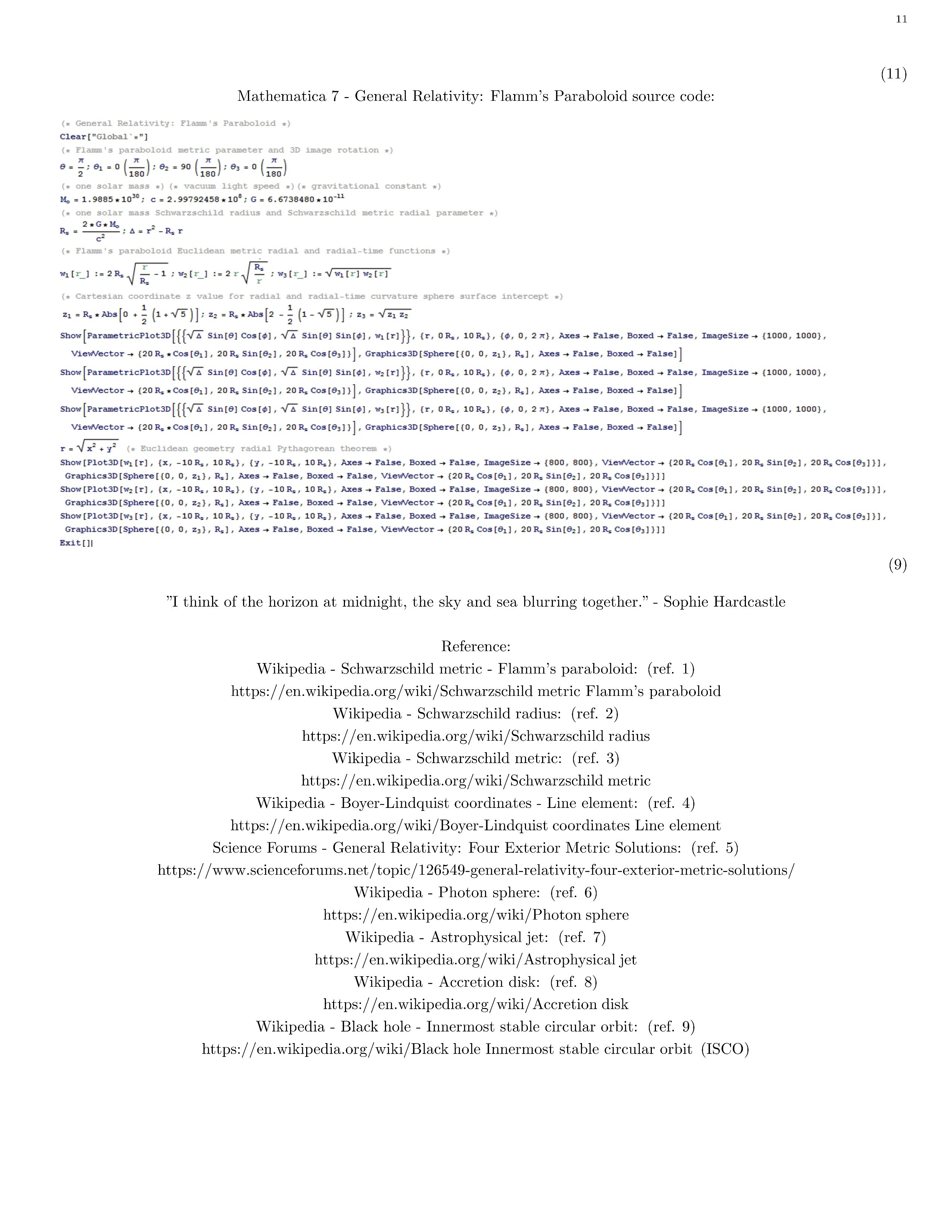
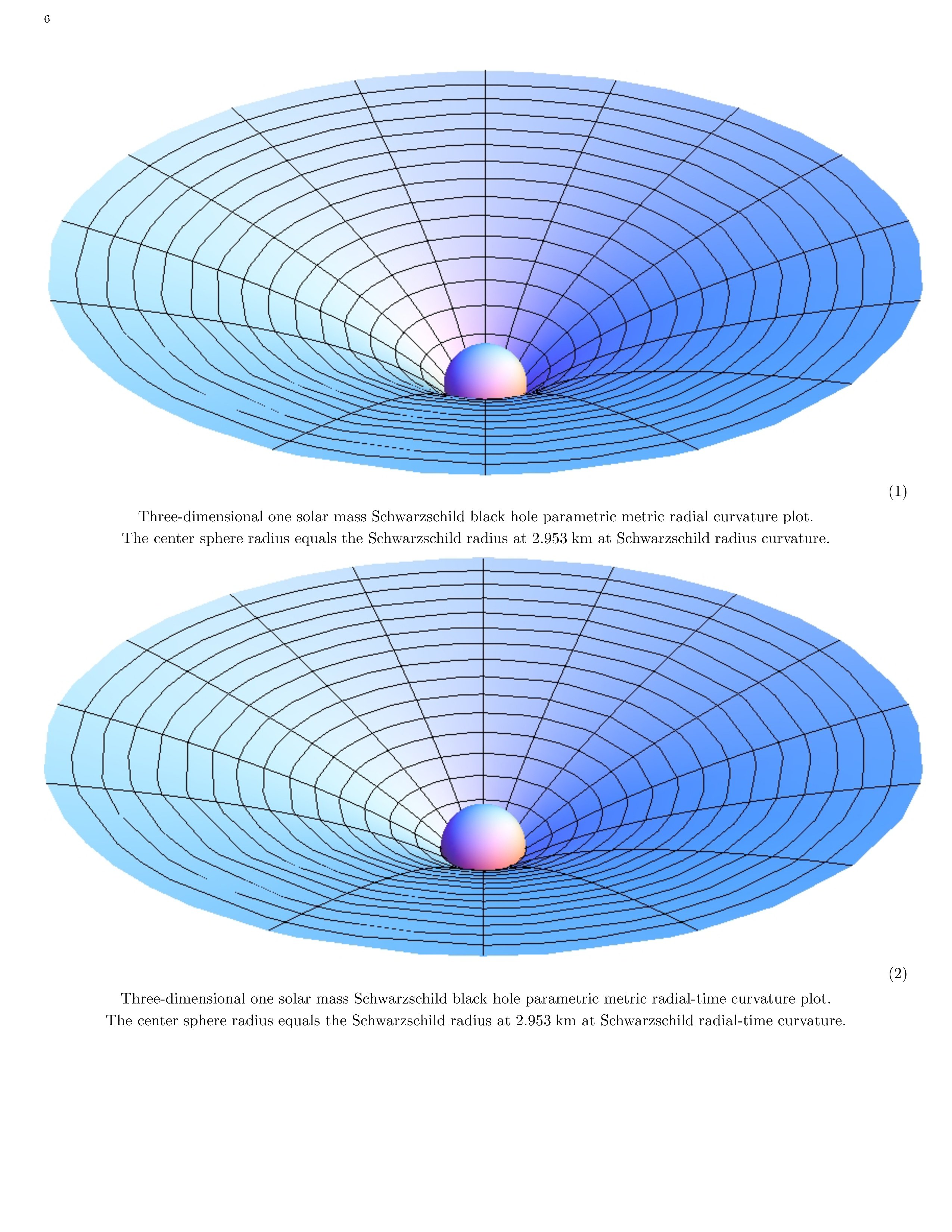
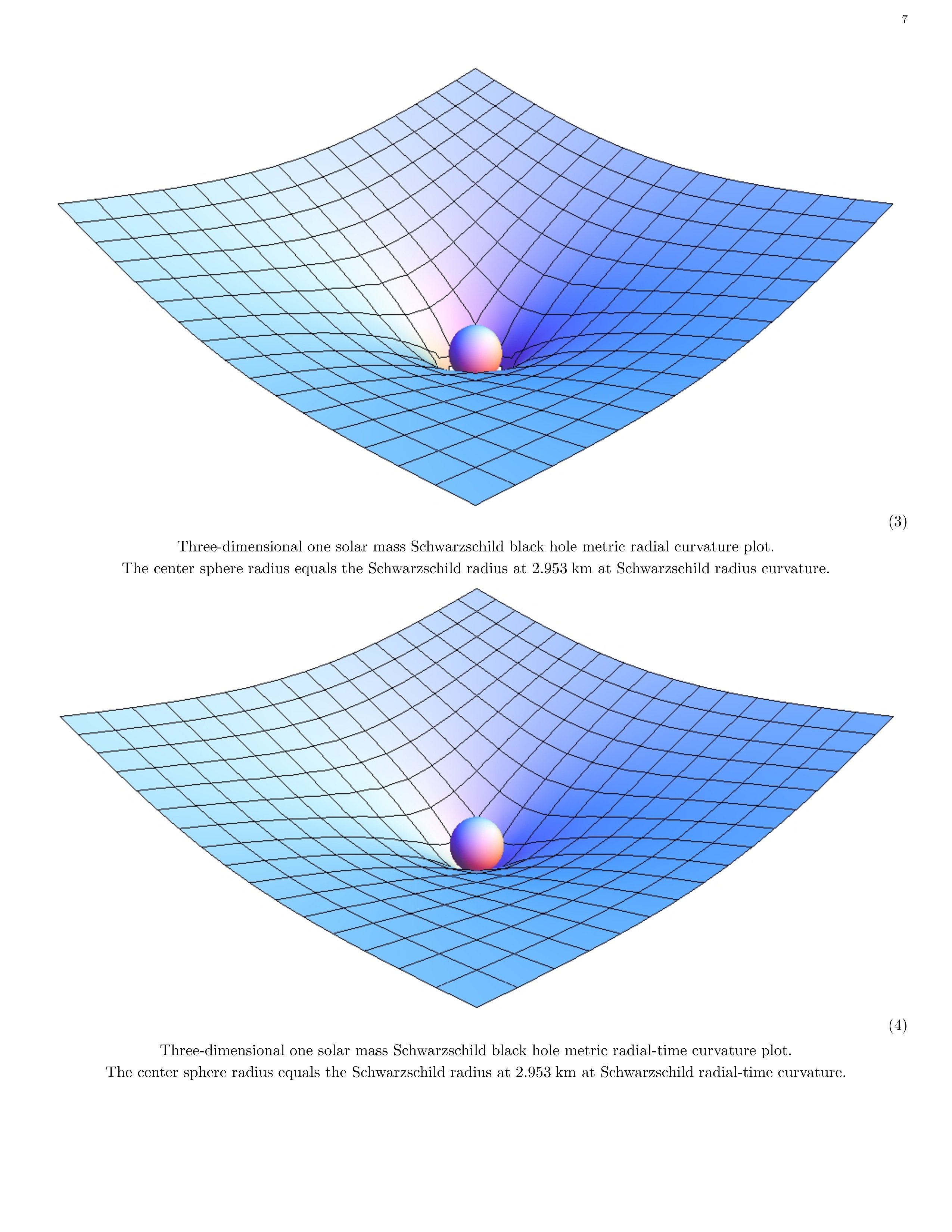

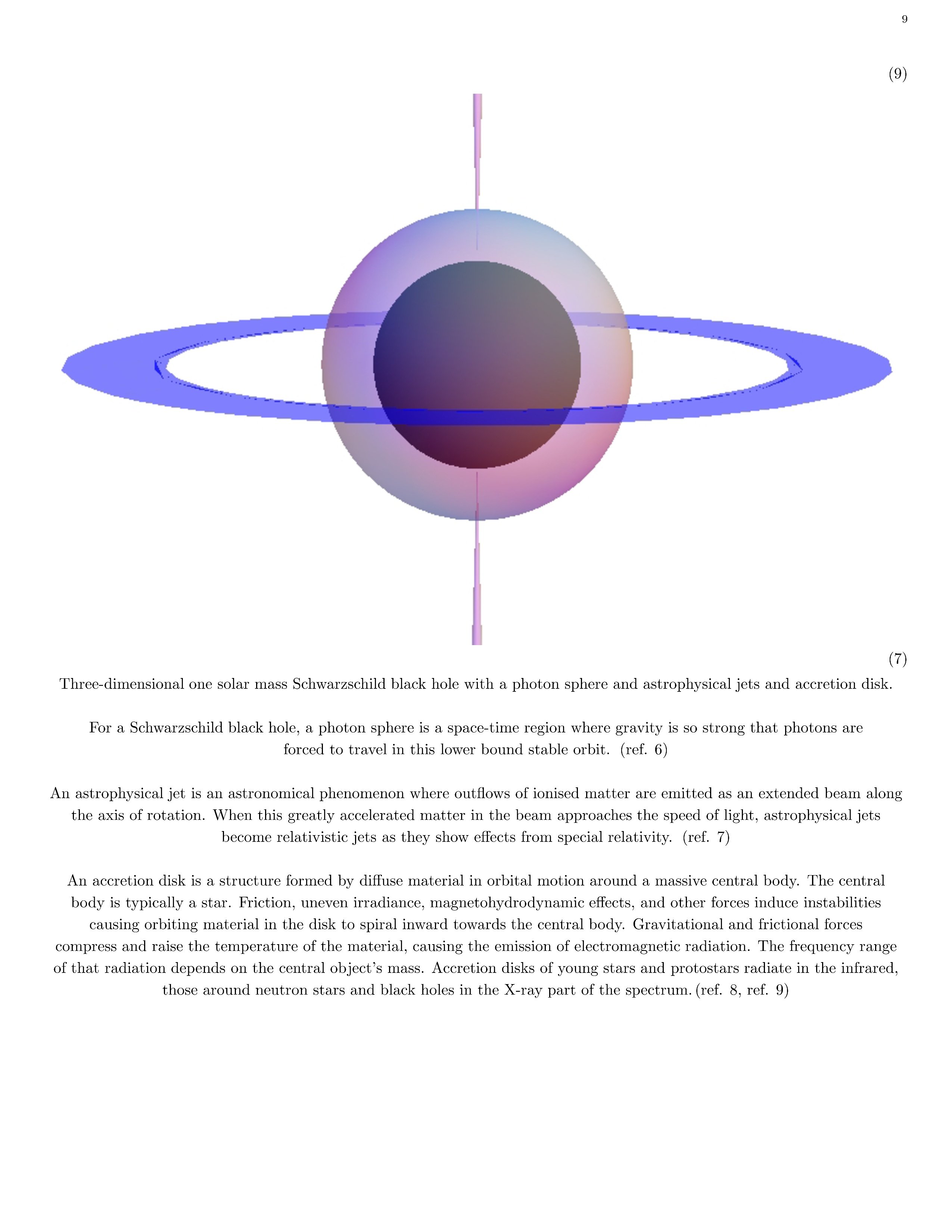


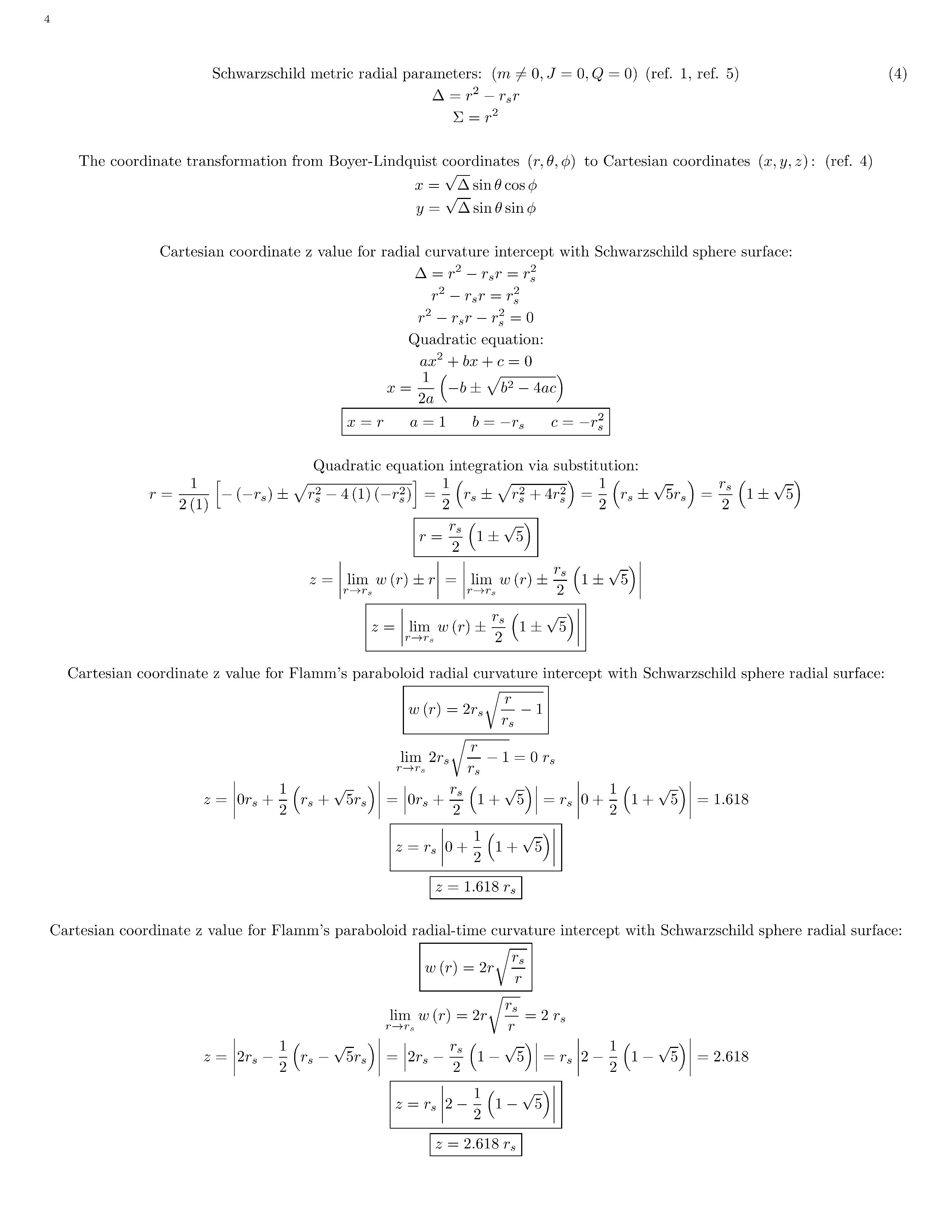
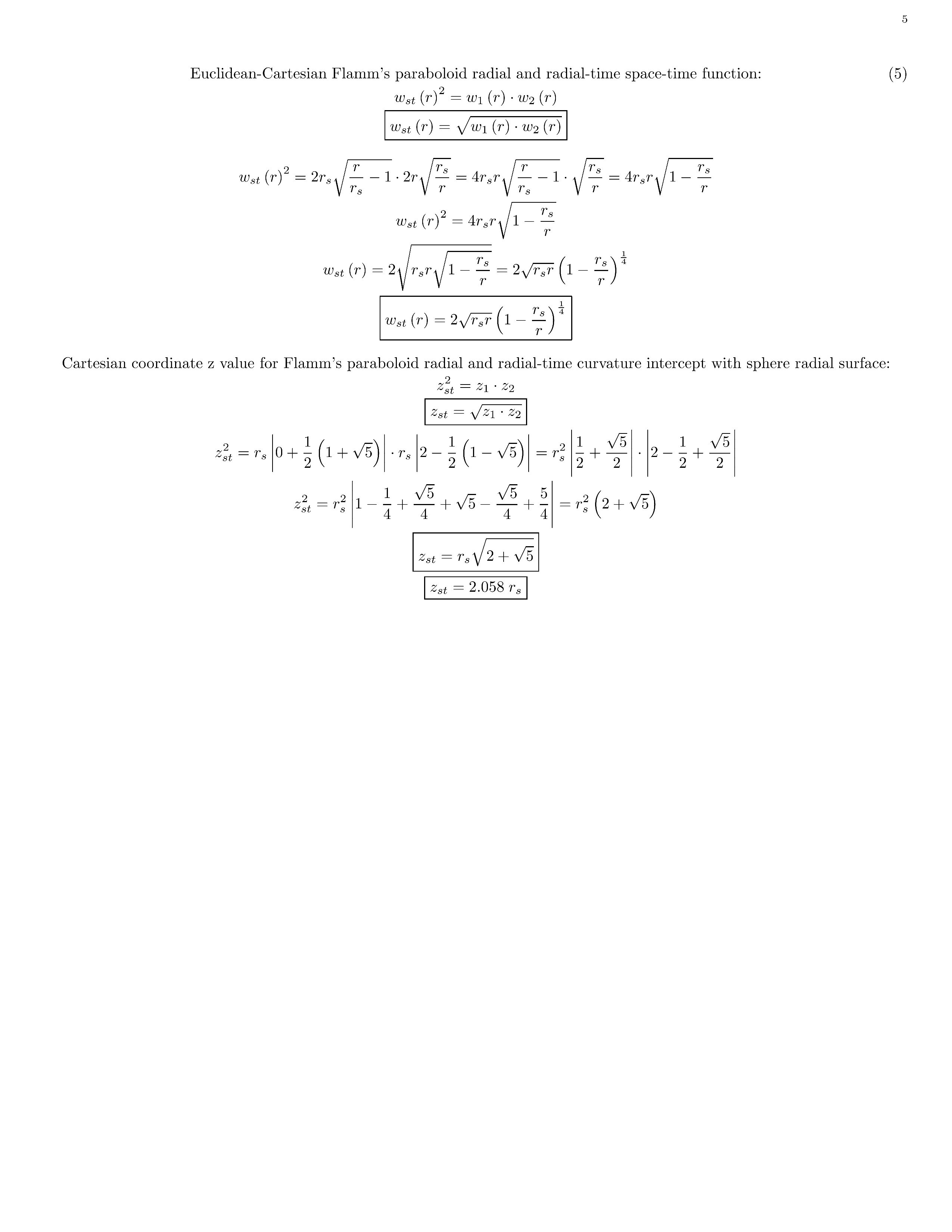
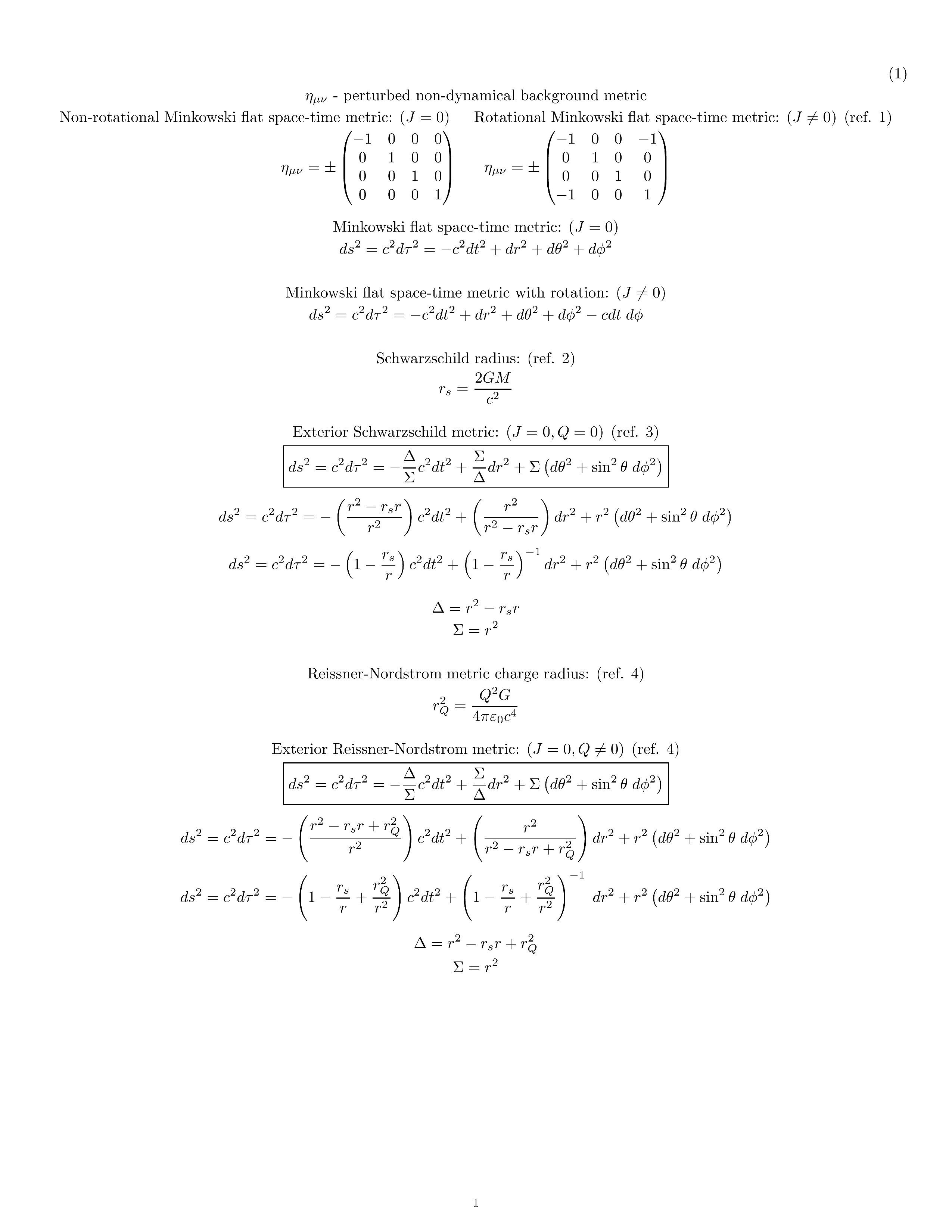
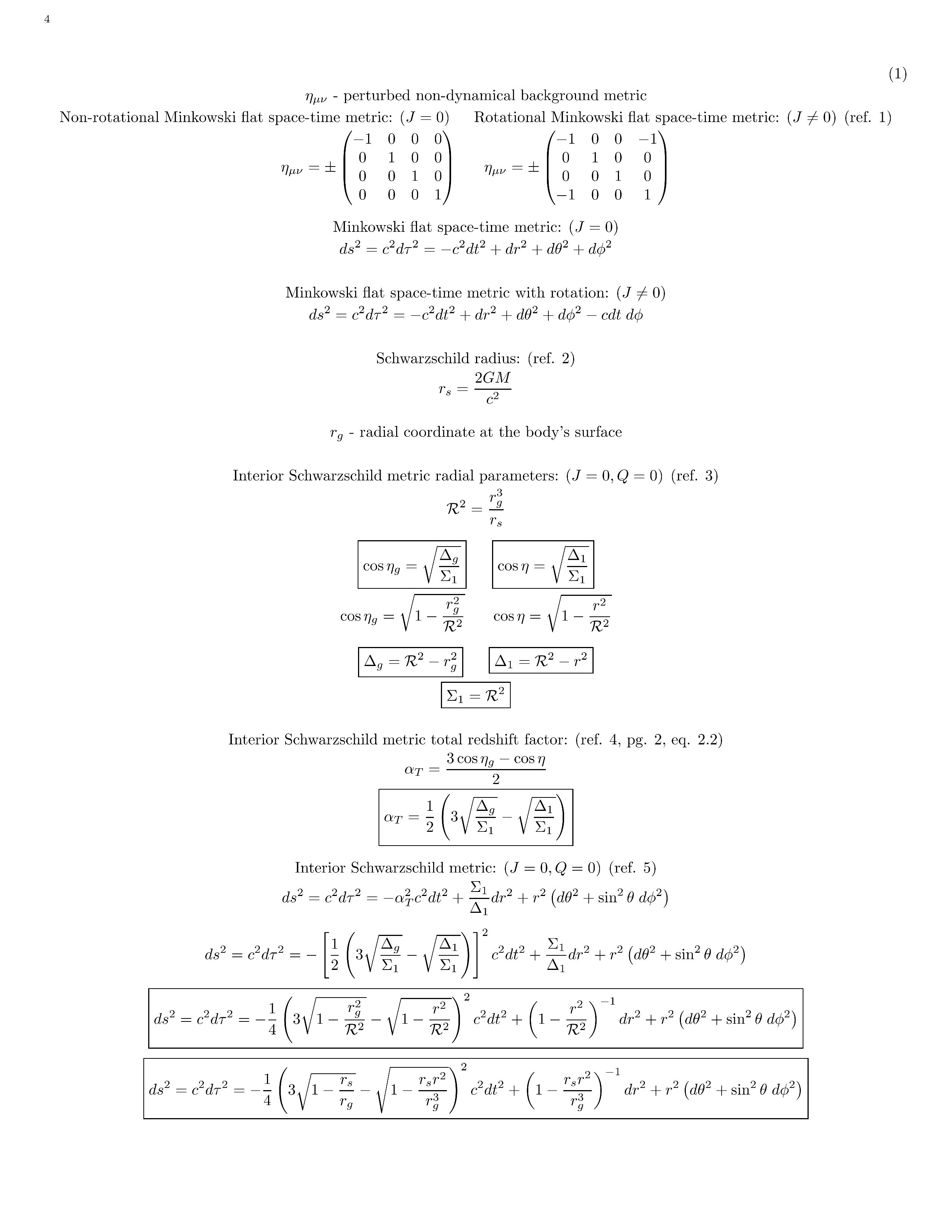
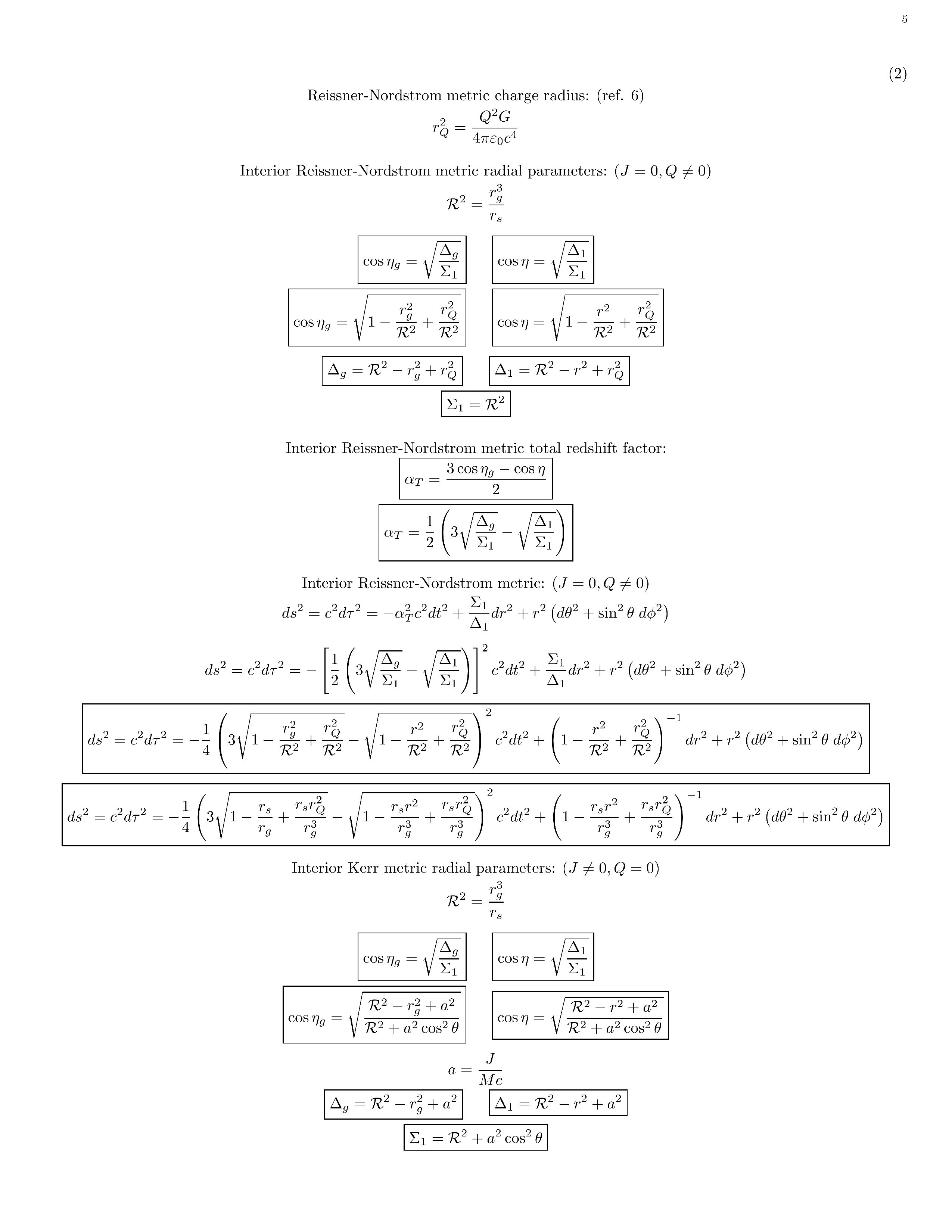
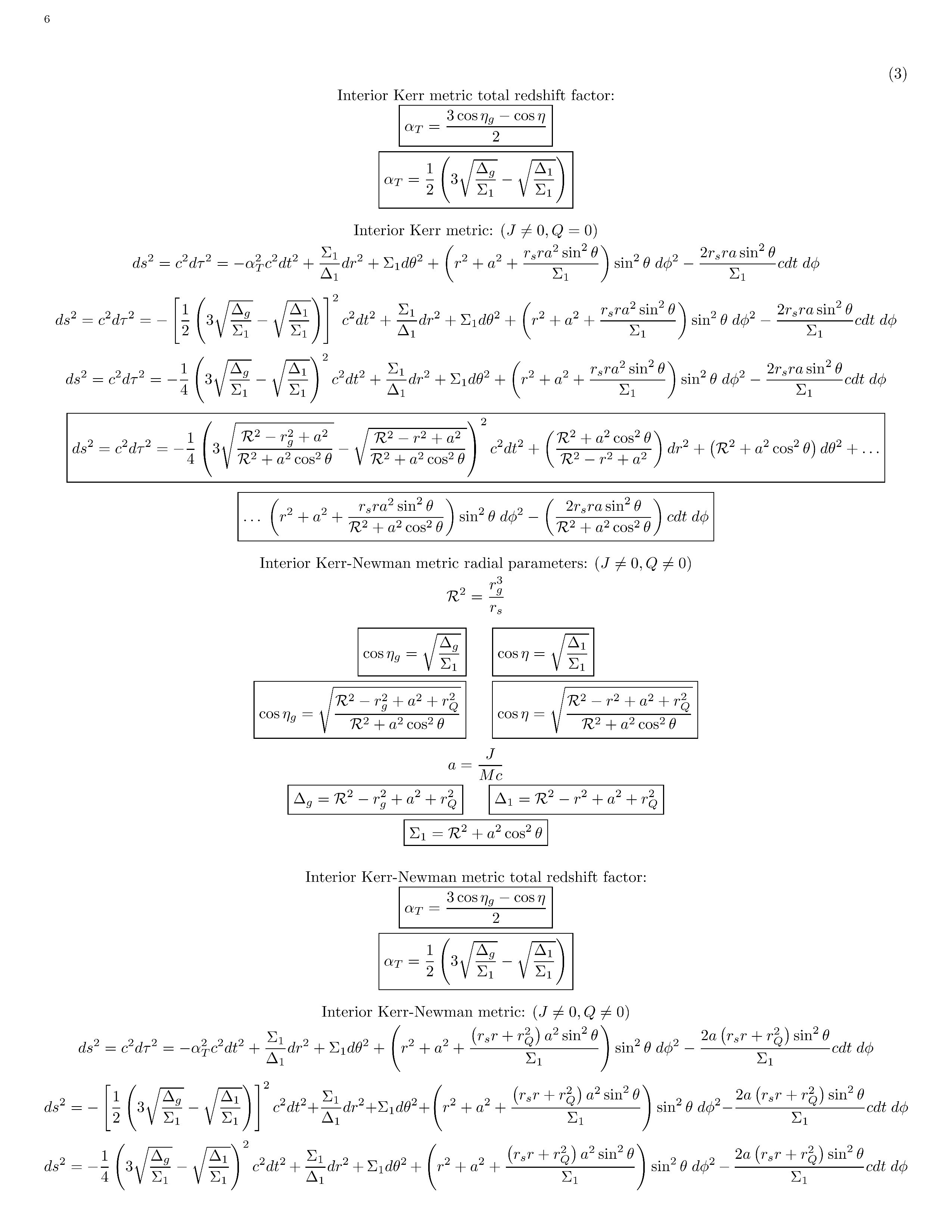
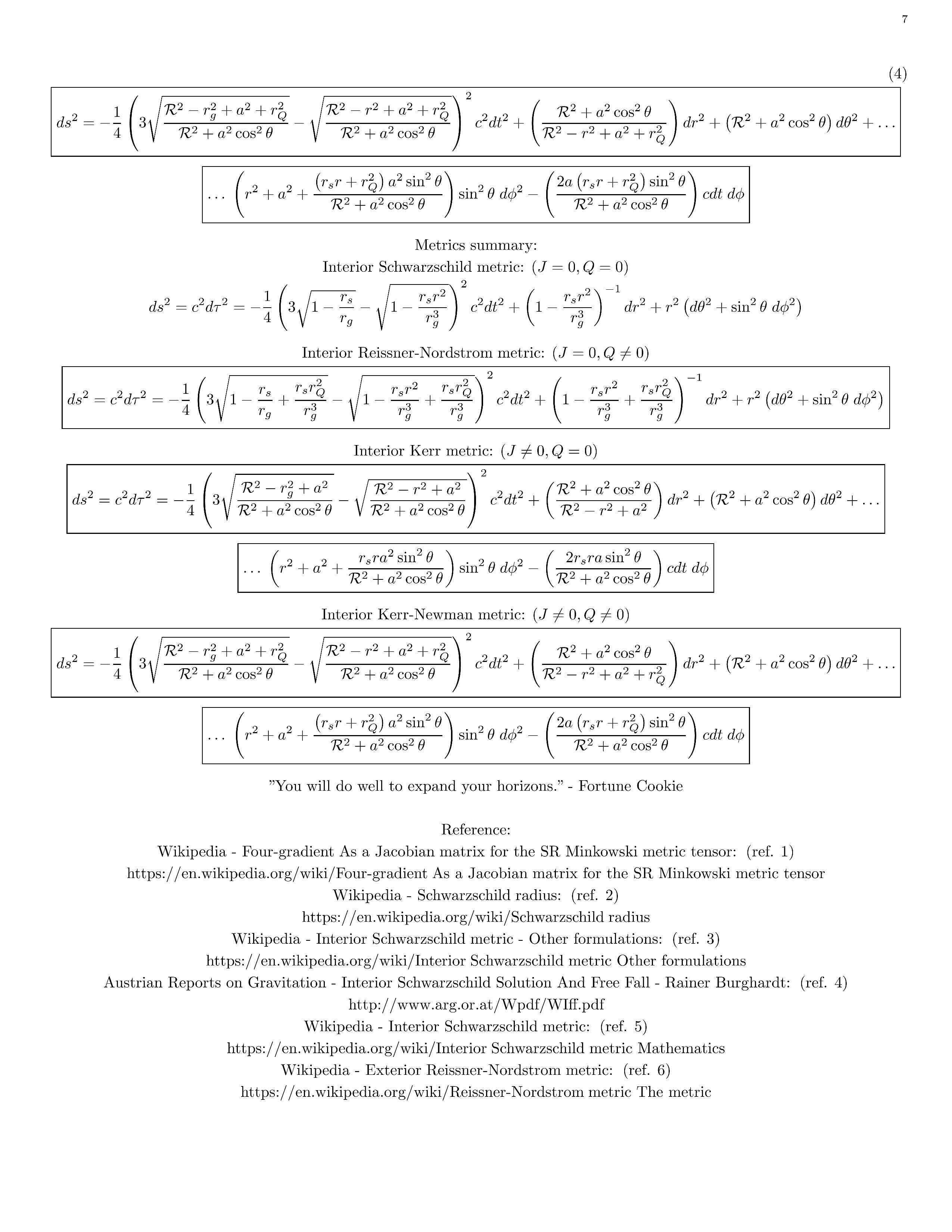
.jpg.3355a0e02727acf7b12833b7133b4cd5.jpg)