Anton Rize

I notice you completely ignored the empirical data, the SPARC RAR graph, and the Wide Binary tests demonstrating 0-parameter accuracy, choosing instead to retreat to elementary geometry. But I will humor your question. Also you still ignoring my goal pole question. You have to admit it not to me but to yourself: If your believes unfalsifiable then they are NOT scientific. Yes, plain and simple: if you graph [math]y = 4\pi r^2[/math] against [math]r[/math], you get a parabola. Yes, the topological [math]S^2[/math] carrier possesses the exact metric area of [math]4\pi r^2[/math]. If you leading me to: "Since it is a 3D sphere, it must enclose a volume of [math]\frac{4}{3}\pi r^3[/math], therefore your density equation is missing the [math]1/3[/math] factor!" Let me stop you right there and refer you back to the ontology you refuse to read. In classical Euclidean space, a sphere is a boundary enclosing a physical volumetric void that gets filled with a fluid. In WILL Relational Geometry, the [math]S^2[/math] carrier is not a container; it is the geometric capacity of the potential projection itself. The energy state is the surface projection ([math]\kappa^2[/math]). There is no independent "inside volume" to integrate over. That is exactly why the algebraic closure in my model is strictly [math]m_0 = 4\pi r^3 \rho[/math], without Newtonian [math]1/3[/math] fluid coefficient. Now that I have answered your geometry question, are you going to address my goal pole question and the physical rotation curves + the Wide Binary data I just provided, or are we going to continue plotting parabolas?

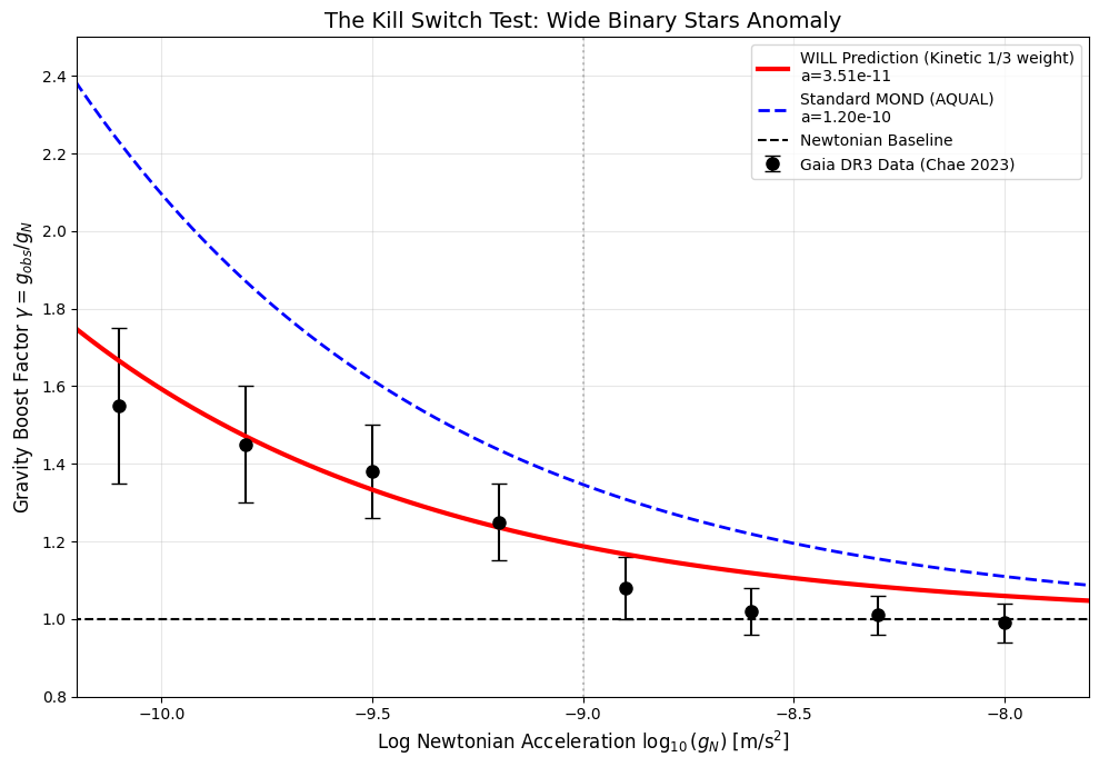
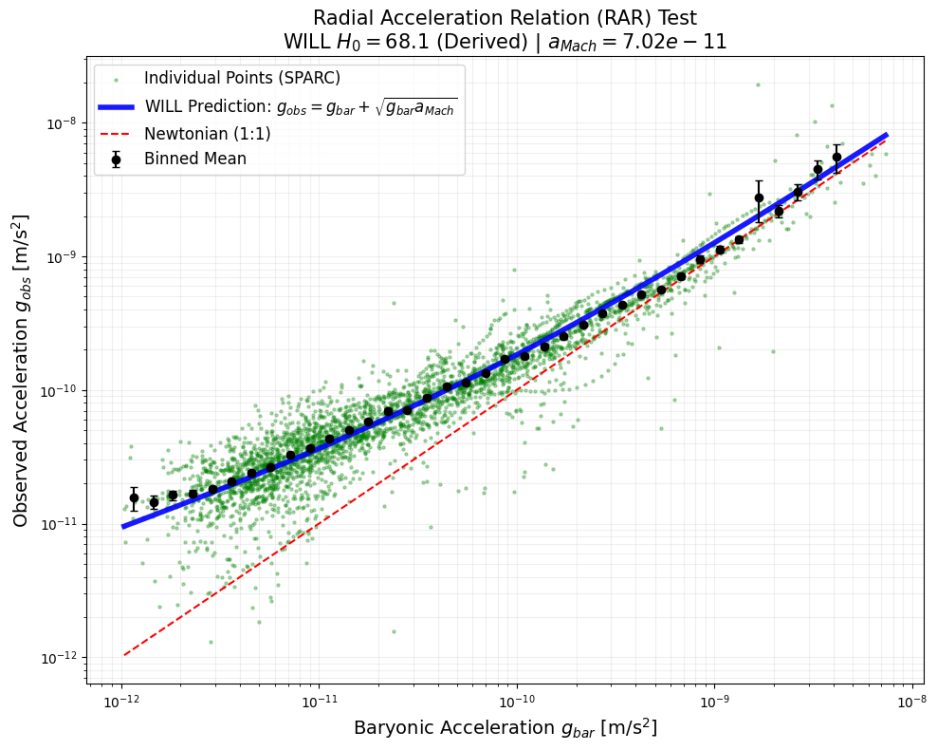
You asked exactly the right question: "how do you explain the discrepancy between rotation velocity in the outer of the Galaxy and the inner region?" In standard cosmology, because the Newtonian velocity drops off as [math]1/\sqrt{r}[/math], they have to invent a halo of invisible mass (Dark Matter) that grows with [math]r[/math] to keep the rotation curve flat. In WILL Relational Geometry, the explanation requires zero invisible particles and no adjustable parameters. It is a direct consequence of SPACETIME ≡ ENERGY. I will show it in 4 steps: Step 1 The Necessity of Global Resonance Step 2 Deriving [math]H_0[/math] from CMB Temperature and [math]\alpha[/math] Step 3 The Resonant Horizon Interference Step 4 Derivation of the Baryonic Tully-Fisher Relation All this leads us to conclusion: The discrepancy in the outer regions of the galaxy is not caused by "missing mass." It is the physical manifestation of the star hitting the energetic floor (the Fundamental Tone) supported by the global resonance of the Universe. It cannot slow down any further because it is coupled to the horizon. To make sure that everyone could test it against empirical data I developed this page https://willrg.com/Galactic_Dynamics/ Its an interactive LAB where you can calculate rotation speed of any galaxy in SPARC database (175 total). This page development was a peace of work I have to admit. Hope you will find it useful. Also here's RAR graph: Radial Acceleration Relation (RAR) for 175 SPARC galaxies. The green dots shows the density of [math]>3000[/math] individual data points. The cyan line represents the WILL Resonance Interference prediction ([math]g_{obs} = g_{bar} + \sqrt{g_{bar}a_{\kappa}}[/math]) using the [math]H_0[/math] value derived from CMB thermodynamics. The remarkable agreement ([math]RMSE \approx 0.065[/math] dex) without free parameters strongly suggests that galactic dynamics are regulated by the global horizon. Colab notebook link: [RAR test.ipynb](https://github.com/AntonRize/WILL/blob/8967a5fac8a7a42433e9cc66fffbbbbc4e18b6a1/Colab_Notebooks/RAR_test.ipynb) And here's the wide binary stars graph based on Gaia DR3 catalog where we comparing WILL and MOND: The Kinetic Resonance Test. The plot compares the gravity boost factor as a function of Newtonian acceleration. Blue dashed line: Standard MOND prediction ([math]a_0 = 1.2 \times 10^{-10} m/s^2[/math]), which systematically overestimates the anomaly. Red solid line: WILL RG Kinetic Resonance prediction ([math]a_{\beta} = cH_0/6\pi \approx 0.35 \times 10^{-10} m/s^2[/math]) passes precisely through the observational data points, matches the reported trend of Wide Binary observations without any parameter fitting. Colab notebook link: [Wide binary Chae 2023.ipynb](https://github.com/AntonRize/WILL/blob/8967a5fac8a7a42433e9cc66fffbbbbc4e18b6a1/Colab_Notebooks/Wide_binary_Chae_2023.ipynb) You can find all my derivations and all my python scripts on this page: https://willrg.com/results/

There is no single geometric object with an area of [math]8\pi r^2[/math]. The number 8 is simply the result of multiplying 4 by 2. Please look closely at the two lines of the derivation I posted: Line 1: [math]\rho = \frac{1}{4\pi} \left( \frac{\kappa^2 c^2}{2 G r^2} \right)[/math] Line 2: [math]\rho = \frac{\kappa^2 c^2}{8\pi G r^2}[/math] The [math]4\pi[/math] in the denominator is the normalization factor from the [math]S^2[/math] carrier area. The [math]2G[/math] in the denominator comes from the mass scale factor ([math]R_s = 2GM/c^2[/math]). When you multiply the denominators, [math]4\pi \times 2G = 8\pi G[/math]. I am not "switching" terms. I am executing basic algebraic multiplication. Does this clarify the geometry for you?

Sorry Im not following where you leading with this. Can you elaborate please?

What do you mean " without explaining why" ? "To translate this into a volumetric density, we first adopt the conventional 3D (volumetric) proxy, [math]r^3[/math]. This is not a postulate of RG, but the first step in applying the legacy (3D) definition of density: [math]\frac{m_0}{r^3} = \frac{\kappa^2 c^2}{2G r^2}[/math] This expression, however, is incomplete. Our [math]\kappa^2[/math] "lives" on the 2D surface [math]S^2[/math] (which corresponds to [math]4\pi[/math]), while the [math]r^3[/math] proxy implicitly assumes a 3D volume. To correctly normalize the 2D parameter [math]\kappa^2[/math] against the 3D volume, we must apply the geometric normalization factor of the [math]S^2[/math] carrier by dividing by the area of the sphere, which introduces the factor [math]\frac{1}{4\pi}[/math]. This normalization is the necessary geometric step to interface the 2D relational carrier ([math]S^2[/math]) with the 3D legacy definition of density: [math]\rho = \frac{1}{4\pi}( \frac{\kappa^2 c^2}{2G r^2} )[/math] [math]\rho = \frac{\kappa^2 c^2}{8\pi G r^2}[/math] [math]\text{Local Density} \equiv \text{Relational Projection}[/math]" Please specify what exactly seems unclear to you?

Welcome back @joigus ! I will assume that you came not just to drop a comment but also to engage in conversation. So Ill gladly provide you with transparent derivations of Lagrangian and Hamiltonian. Next in line is Newtons third law you can find here https://willrg.com/documents/WILL_RG_I.pdf#thm:third_law We now demonstrate that the familiar Lagrangian and Hamiltonian formalisms arise as limiting cases of the two-point relational Energy-Symmetry Law. Specifically, they emerge when the relational structure between two distinct observers A and B is collapsed into a single-point local description. This collapse preserves computational utility but reduces the ontological transparency of the underlying relational structure. Definitions of Parameters We consider a central mass [math]M[/math] and a test mass [math]m[/math]. The state of the test mass is described in polar coordinates [math](r,\phi)[/math] relative to the central mass. * [math]r_A[/math] --- reference radius associated with observer A (e.g., planetary surface). * [math]r_B[/math] --- orbital radius of the test mass [math]m[/math] (position of observer B). * [math]v_B^2 = \dot r_B^2 + r_B^2 \dot\phi^2[/math] --- total squared orbital speed at B. * [math]\beta_B^2 = v_B^2/c^2[/math] --- dimensionless kinematic projection at B. * [math]\kappa_A^2 = 2GM/(r_A c^2)[/math] --- dimensionless potential projection defined at A. The Relational Lagrangian Instead of a relational energy, we define the clean relational Lagrangian [math]L_{rel}[/math], which represents the kinetic budget at point B relative to the potential budget at point A: [math]L_{rel} = T(B) + U(A) = \frac{1}{2} m(\dot r_B^2 + r_B^2 \dot\phi^2) + \frac{GMm}{r_A}[/math] In dimensionless form, using the rest energy [math]E_0 = mc^2[/math], this is: [math]\frac{L_{rel}}{E_0} = \frac{1}{2}(\beta_B^2 + \kappa_A^2)[/math] This two-point, relational form is the clean geometric statement. First Ontological Collapse: The Newtonian Lagrangian If one commits the first ontological violation by identifying the two distinct points, [math]r_A = r_B = r[/math], the relational structure degenerates into a local, single-point function: [math]L(r,\dot r,\dot\phi) = \frac{1}{2} m(\dot r^2+r^2\dot\phi^2) + \frac{GMm}{r}[/math] This is precisely the standard Newtonian Lagrangian. Its origin is not fundamental but arises from the collapse of the two-point relational Energy Symmetry law into a one-point formalism. Second Ontological Collapse: The Hamiltonian Introducing canonical momenta, [math]p_r = \frac{\partial L}{\partial \dot r} = m\dot r[/math] [math]p_\phi = \frac{\partial L}{\partial \dot\phi} = mr^2\dot\phi[/math] one defines the Hamiltonian via the Legendre transformation [math]H = p_r \dot r + p_\phi \dot\phi - L[/math]. This evaluates to the total energy of the collapsed system: [math]H = T+U = \frac{1}{2} m(\dot r^2 + r^2 \dot\phi^2) + \frac{GMm}{r}[/math] Interpretation In terms of the collapsed WILL projections ([math]\beta^2 = v^2/c^2[/math] and [math]\kappa^2 = 2GM/(rc^2)[/math], both strictly positive), the match to standard mechanics becomes explicit: [math]L = \frac{1}{2} m v^2 + \frac{GMm}{r} \longleftrightarrow \frac{1}{2} m c^2(\beta^2 + \kappa^2)[/math] [math]H = \frac{1}{2} m v^2 - \frac{GMm}{r} \longleftrightarrow \frac{1}{2} m c^2(\beta^2 - \kappa^2)[/math] Here the "+" or "-" signs do not come from [math]\kappa^2[/math] itself, which is always positive, but from the ontological collapse of the two-point relational energy law into a single-point formalism. In WILL, both projections are clean and positive; in standard mechanics, the apparent sign difference arises only after this collapse. Both the Lagrangian and Hamiltonian thus emerge from the same relational Energy-Symmetry Law under the identification [math]r_A = r_B = r[/math]. The apparent sign difference between [math]L[/math] and [math]H[/math] is not a fundamental feature but an artifact of this single-point collapse: in the full two-point relational law, both projections [math]\beta^2[/math] and [math]\kappa^2[/math] are strictly positive. The Lagrangian and Hamiltonian arise as single-point limiting cases of the two-point relational Energy-Symmetry Law [math]\Delta E_{A\to B} + \Delta E_{B\to A} = 0[/math]. They remain computationally valid within their domain of applicability. RG provides the more general two-point relational structure from which these formalisms can be systematically derived.

You have raised a crucial philosophical point, but I must respectfully disagree with your underlying premise. You are conflating mathematical flexibility with physical constraint. Discoveries like Neptune were not made because the model was "flexible." They were made precisely because classical mechanics was rigid. When the orbit of Uranus violated predictions, Le Verrier did not have the "flexibility" to alter Newton's gravitational constant or invent a new force distance parameter. Because the model's constraints were absolute, the anomaly strictly demanded a localized physical explanation. That rigidity is exactly what pointed the telescope at Neptune. If a model is "flexible" enough that you can just add a mathematical parameter every time an observation deviates from theory (like adding epicycles, or adding an invisible "Dark Matter" halo to fix a galactic rotation curve), you stop looking for physical reality. You just fit the curve. Flexibility is often the enemy of discovery; it hides structural failures under mathematical patches. This brings me to your comment about my math. You suggested that my model "incorporates Hamiltonian, Klein Gordon equations... and manipulation of physics units/SI units in a smart way" to give short answers. I need to be absolutely clear: it does not. There are no hidden quantum mechanical operators, no Hamiltonians, and no dimensional juggling under the hood. I'm keeping everything dimensionless at all times and units used only when its absolutely necessary. The reason the derivations are so short and direct is that the framework relies entirely on generative geometric constraints, not phenomenological equations. Hamiltonian same as Lagrangian are derived: Lagrangian and Hamiltonian as Single-Point Limits of the Relational Energy-Symmetry Law A rigid, zero-parameter model like WILL RG does not prevent the prediction of the unknown. On the contrary: because it has zero flexibility, any future observation that deviates from its predictions cannot simply be "patched" with a new parameter. It will immediately expose the exact location of actual new physics or exact limitation of the current model. There's no place for dark sector in RG. Ok I will copy and paste and convert the formatting of math for you, but you have to explain what difficulties are you facing when clicking on to direct link like this?: https://willrg.com/documents/WILL_RG_I.pdf#sec:density the same derivation from this link Ill provide below: Translating RG (2D) to Conventional Density (3D). In RG [math]\kappa^2[/math] is the 2D parameter defined in the relational carrier [math]S^2[/math]. In conventional physics, the source term is volumetric density [math]\rho[/math], a 3D concept defined by the "cultural artifact" (a Newtonian "cannonball" model) of mass-per-volume. To bridge our 2D theory with 3D empirical data, we must create a "translation interface". We do this by explicitly adopting the conventional (Newtonian) definition of density, [math]\rho \propto m_0/r^3[/math], as our "translation target". From the projective analysis established in the previous sections: [math]\kappa^2 = \frac{R_s}{r}[/math] where [math]\kappa[/math] emerges from the energy projection on the area of unit sphere [math]S^2[/math], and [math]R_s = \frac{2Gm_0}{c^2}[/math] links to the mass scale factor [math]m_0 = \frac{E_0}{c^2}[/math]. This leads to mass definition: [math]m_0 = \frac{\kappa^2 c^2 r}{2G}[/math] To translate this into a volumetric density, we first adopt the conventional 3D (volumetric) proxy, [math]r^3[/math]. This is not a postulate of RG, but the first step in applying the legacy (3D) definition of density: [math]\frac{m_0}{r^3} = \frac{\kappa^2 c^2}{2G r^2}[/math] This expression, however, is incomplete. Our [math]\kappa^2[/math] "lives" on the 2D surface [math]S^2[/math] (which corresponds to [math]4\pi[/math]), while the [math]r^3[/math] proxy implicitly assumes a 3D volume. To correctly normalize the 2D parameter [math]\kappa^2[/math] against the 3D volume, we must apply the geometric normalization factor of the [math]S^2[/math] carrier by dividing by the area of the sphere, which introduces the factor [math]\frac{1}{4\pi}[/math]. This normalization is the necessary geometric step to interface the 2D relational carrier ([math]S^2[/math]) with the 3D legacy definition of density: [math]\rho = \frac{1}{4\pi}( \frac{\kappa^2 c^2}{2G r^2} )[/math] [math]\rho = \frac{\kappa^2 c^2}{8\pi G r^2}[/math] [math]\text{Local Density} \equiv \text{Relational Projection}[/math] Maximal Density. At [math]\kappa^2 = 1[/math] (the horizon condition (for non rotating systems), [math]r=R_s[/math]), this density reaches its natural bound, [math]\rho_{\max}[/math], which is derived purely from geometry: [math]\rho_{\max} = \frac{c^2}{8\pi G r^2}[/math] Normalized Relation. Thus, our "translation" reveals an identity: the geometric projection [math]\kappa^2[/math] is simply the ratio of density to the maximal density: [math]\kappa^2 = \frac{\rho}{\rho_{\max}} \rightarrow \kappa^2 \equiv \Omega[/math] Self-Consistency Requirement The mass scale factor can be expressed in two equivalent ways. From the geometric definition: [math]m_0 = \frac{\kappa^2 c^2 r}{2G}[/math] From the energy density: [math]m_0 = \alpha r^n \rho[/math] Substituting [math]\rho = \frac{\kappa^2 c^2}{8\pi G r^2}[/math] into [math]m_0 = \alpha r^n \rho[/math] gives: [math]m_0 = \frac{\alpha \kappa^2 c^2 r^{n-2}}{8\pi G}[/math] Equating the two forms: [math]\frac{\alpha r^{n-2}}{8\pi} = \frac{r}{2}[/math] For the mass [math]m_0[/math] to remain a constant independent of the measurement scale [math]r[/math], the exponent must be [math]n=3[/math], yielding [math]\alpha=4\pi[/math]. Hence: [math]m_0 = 4\pi r^3 \rho[/math] which closes the consistency loop between the geometric and density-based formulations.

I have to admit that this is a completely new experience to me - you are the first person in this 250+ comments thread who is not dismissing my ontology... I didn't realize how horribly sad it is until I typed it out... I also would like to emphasize the redefinition of energy wasn't my philosophical choice. The standard "ability to do work" - violates the principle of relational origin. So my definition, same as everything else in my research is forced by the core method that Im committed to. If my research ever finds wider acceptance it is this generative method of mine I consider the biggest contribution. It shows a different way to do science where ontology comes first. No mindless phenomenology no curve fitting no unfalsifiable models. P.S. I would be very curious to hear your "controversial" definition - it seems our intuitions are vibrating on the same frequency.

According to my results in https://willrg.com/documents/WILL_RG_II.pdf The vast majority (only week lensing left unsolved; just haven't touched it yet) of observational phenomena that we interpreting as DE, DM are inevitable consequents of Relational Geometry. We just don't have to speculate any "dark" entities to accurately predict and explain observables. The “missing mass” is not missing mass. It is the observable signature of a star’s resonant coupling to the cosmic horizon inside a closed relational geometry. Dark Matter becomes redundant. CRITICAL NOTE: Regardless of complete publicity of all data and tools and methodological discipline of my Open Research - My results are still remain unverified independently. Until independent verification is confirmed we should avoid such categorical formulations: "dark matter doesn't exist".

That is a very vague redirection. 1. On the Math: Could you be specific? Which exact RG equation violates which rule of inner or cross-product addition? [math]\kappa^2[/math] is explicitly derived as the square of a relational projection (inner product geometry) on an [math]S^2[/math] carrier (cross-product area geometry). Dropping terms like "vector addition rules" without showing a specific algebraic contradiction is not a critique; it is a distraction. 2. On the Logic: You completely avoided my primary question. I will ask it again: What are your specific, objective criteria for a model to be taken seriously? I have derived [math]H_0[/math] with zero parameters, solved the orbital degeneracy problem, and computed the recombination epoch. If these results are not enough, what is? Do you have a defined threshold for evidence, or are you simply going to throw random jargon from a physics textbook every time the derivation holds up? You are attempting to judge a fundamental generative geometry using the secondary mathematical artifacts of a 100-year-old descriptive model. 1. On "Inner Products" and "Vector Rules": These are not physical laws; they are bookkeeping tools designed for 3D Euclidean containers. An inner product requires a pre-defined metric space to exist. RG does not assume a metric space - it generates one from the relational energy projections (alpha, light wavelength) things we can physically measure. You trying to legitimize unphysical unmeasurable model specific mathematical tools. Using vector addition rules to "correct" RG is like trying to use a thermometer to measure the volume of a shadow. It is a category error. 2. Observed Reality vs. Tensors: The Stress-Energy Tensor (Tμν) is an ad-hoc mathematical construct used to balance equations in a fluid-dynamic model that requires Dark Matter to function. RG operates on physical observables: absolute temperatures, coupling constants, and geometric closure limits. 3. The Goalpost Question: You have repeatedly retreated into textbook jargon to avoid a simple fact: RG produces accurate physical results (H0, recombination, orbital tests and many more) with zero free parameters - results your "3 methodologies" can only achieve by "throwing in" invisible dark substances. I will not waste more time debating the commutative properties of your mathematical "toys." If you have a specific physical observation that contradicts the output of my equations, present it. If not, then your critique is nothing more than a defense of a map that is no longer the territory. What is your objective threshold for a model to be valid? Does it have to be true, or does it just have to use your favorite tensors? Is your physical believes based on dogmas or scientific principals?

Its just an misunderstanding. The [math]1/R^2[/math] dependence in the critical density formula is not a sign of "2-dimensionality." It is the signature system at its saturation limit. In standard physics, density is [math]M/R^3[/math]. The only reason the critical density scales as [math]1/R^2[/math] is because at the horizon, the mass of the Universe scales linearly with radius ([math]M \propto R[/math]). This linear growth of mass cancels one power of the cubic volume, leaving [math]R/R^3 = 1/R^2[/math]. In RG, this isn't a "coincidence" - it is derived. The density still has 3DOF: [math]\rho = \frac{R_s c^2}{8\pi G r^3} = \frac{\kappa^{2}c^{2}}{8\pi Gr^{2}} [/math] [math] \rho_{max}=\frac{c^{2}}{8\cdot\pi\cdot G\cdot r^{2}} [/math] However, because [math]\kappa^2 = R_s/r[/math], at the horizon (where [math]\kappa^2 = 1[/math] and [math]r = R_s[/math]), the "invisible" [math]R_s[/math] in the numerator cancels one [math]r[/math] in the denominator. You are looking at the residue of a r^3 -> r^2 cancellation. But let's step back from moving goalposts. I want to ask you directly: What are your specific, objective criteria for a model to be taken seriously? 1. Derive [math]H_0[/math] from [math]T_0[/math] and [math]\alpha[/math] with zero free parameters? (Done). 2. Solve the parameter degeneracy in orbital mechanics? (Done). 3. Derive the recombination epoch without Dark Matter? (Done). Is there a threshold of mathematical evidence that would shift your stance from "dismissing the derivation" to "engaging with the ontology," or are the goalposts intended to stay in motion indefinitely?

Thank you for posting this exact derivation. This is the perfect pedagogical moment, because it highlights the precise ontological divergence between the Standard Model and WILL RG in a single line. Look carefully at the third step of your proof: [math] \text{mass} \quad \rho \times \text{volume} = \rho \times \frac{4}{3}\pi R^3 [/math] Where does the factor of 3 come from? It comes exclusively from the geometric formula for the volume of a 3D sphere. Your derivation explicitly assumes that the Universe is an expanding Newtonian 3D container filled with a uniform fluid/dust. This is the classical derivation of the Friedmann equation. Now, please look at the section in my paper titled "Self-Consistency Requirement" and the subsection "No Singularities, No Hidden Regions". https://willrg.com/documents/WILL_RG_I.pdf#sec:no_singularities RG strictly forbids the "Newtonian cannonball" volume assumption. The geometric limit is defined by the energy projection on the 2D surface of the [math]S^2[/math] carrier (which carries the [math]4\pi[/math] metric). As derived in the text, the algebraic closure in WILL RG is: [math]m_0 = 4\pi r^3 \rho[/math] There is no [math]1/3[/math] volume coefficient because the geometry is a 2D surface-scaled projection, not a 3D volume integration. If my final equation for [math]H_0[/math] contained that factor of 3, it would mean my mathematics were broken - it would mean I had accidentally smuggled a 3D Newtonian fluid assumption into a 2D relational geometry. The fact that the 3 is missing is not an error; it is the mathematical proof that the topology successfully maintained its [math]S^2[/math] projective integrity all the way to the macroscopic horizon. Your derivation is exactly what I "should have" if I were doing standard Newtonian cosmology. But I am not.

@Mordred , I red through the H_0 derivation section again, and realize that while Im providing links to the source density derivation and Im showing mathematically this factor 1/3 difference [math] \rho_{crit} \approx 9.5 \times 10^{-27} [/math]. [math].kg/m^3[/math].; [math]. \rho_{max} \approx \rho_{crit}/3 [/math]. However I never word this difference in this section properly. So Ill add more pronounce accent on the factor 1/3 in this section to avoid any confusions. Thank you for showing me the source of misinterpretation. Its valuable. Oh no I wouldn't expect you to go through the hole thing. That's why I always sharing hyperlinks like this https://willrg.com/documents/WILL_RG_I.pdf#sec:pressure Just click left mouse button on it and it will redirect you to the exact derivation. Just remember if you will use open new tab command - the hyper part will not work and you will see the 1st page of .pdf instead of specific section. It has to be left mouse button only.

Of course they arrive at the same relation - they all share the exact same ontological assumption: that the Universe is an expanding 3D fluid manifold. My methodology strictly forbid such assumptions. Here's the pressure derivation: https://willrg.com/documents/WILL_RG_I.pdf#sec:pressure Sorry the link was broken. I just fixed it.

Let us trace the exact sequence of logical steps you just demonstrated in your comment: 1. You noticed the absence of the 1/3 factor in the density equation. (A correct observation). 2. You immediately concluded this absence was a mathematical error. 3. You concluded that I must be completely unaware of this "error". 4. You concluded that because I am "unaware," the formulas must have been generated by an AI or copied without understanding. 5. Based on this chain of assumptions, you adopted a pedagogical tone ("I will let you see which formula Im referring to") to test my knowledge of my own work. The critical failure in this sequence of assumptions is that you did not read the derivation you are attempting to critique. If you would follow the link to original density derivation which I implicitly include in this section: "In the Normalization Identity (derived in WILL RG I),". Or If you look at Section 6.2 of the WILL RG Part II document, you will find a dedicated subsection explicitly titled: "1. Saturation Identity (no Friedmann factor)". https://willrg.com/documents/WILL_RG_II.pdf#sec:will-friedmann The text directly below it states: "Consequently, the relation between the Hubble parameter and the saturation density is: [math]H_0^2 = 8\pi G \rho_{max}[/math], without the factor of 1/3 that appears in the standard Friedmann equation... The two expressions are numerically identical ([math]\rho_{max} = \rho_{crit}/3[/math]), but their algebraic origins differ fundamentally." The missing (3) is not a typo, nor is it an AI hallucination. It is the central, mathematically proven topological distinction between a 3D thermodynamic fluid expansion (your paradigm) and a 2D geometric carrier saturation (WILL RG). I am always open to rigorous scientific critique. However, attempting to quiz me on an "error" that is explicitly derived and justified in a dedicated section of the very paper you are criticizing is not scientific rigor.

It is difficult to imagine two more fundamentally opposed methodologies. 1. Categorical Difference: The paper you linked proposes an empirical measurement method requiring the filtration of 17 noise parameters over a decade. My method is pure generative geometry - a strict algebraic deduction that culminates in exact equations with ZERO free parameters. 2. It is not a "local" [math]\beta[/math]: I do not use a local kinematic velocity [math]\beta = v/c[/math] to derive the horizon. I use [math]\beta_1 \equiv \alpha[/math] (the fine-structure constant). As mathematically derived in Part III: (https://willrg.com/documents/WILL_RG_III.pdf#eq:beta=alpha), [math]\alpha[/math] is the invariant kinematic projection of the electromagnetic ground state. It is a universal geometric scale, not a local variable. 3. The [math]z=1100[/math] claim: Your assertion that the numbers would not match at [math]z=1100[/math] is factually incorrect. Using the exact same deductive geometry—specifically, the phase transition condition [math]o_{crit} = 1[/math]—the WILL RG framework explicitly calculates the recombination epoch at [math]z_{dec} \approx 1156[/math] and [math]T \approx 3150[/math] K (see Section 4). The geometry works flawlessly across all cosmological scales. 4. "the numbers you used " - No fitted numbers: The "numbers" I use for the density calculations are not local phenomenological fits. They are absolute constants ([math]T_0, \alpha, G, c[/math]). The model does not take numbers from local measurements to fit the Universe; it derives the macroscopic structure of the Universe directly from microphysical invariants. I have to ask: are we looking at the same equation? The derivation in my paper culminates strictly in this exact algebraic form: [math]H_{0}=\sqrt{8\pi G\frac{4\sigma_{SB}T_{CMB}^{4}}{3\alpha^{2}c^{3}}}[/math] There are no Maxwell-Boltzmann distributions in this derivation, nor does it require Bose-Einstein statistics. It is a direct, deterministic algebraic consequence of geometric saturation, not a statistical probability distribution. As for requiring a "volume element being examined" - that is certainly a necessity if one interprets the Universe as a 3D thermodynamic fluid. However, in the generative ontology of WILL RG, the energy capacity is governed strictly by the closed 2D surface topology of the [math]S^2[/math] carrier. The 3D volume is a secondary geometric projection of this surface capacity. This makes the classical thermodynamic assumption of a "3D volume element" structurally redundant for establishing this specific boundary condition.

thank you for sharing the paper. I have read through it. Before I share my detailed thoughts, I want to make sure I am accurately understanding your perspective. Could you elaborate on what specific correlations you see between the methodology proposed in this paper and the derivation of [math]H_0[/math] in RG? What was the logical chain that led you to suggest this paper as a comparison? I genuinely want to understand how you are mapping their method and mine. Can you elaborate please?

@Mordred , first of all, thank you sincerely for taking the time to look through the calculation. I truly appreciate it. I am especially glad you noted that mathematically, the CMB temperature calculation regarding photon density works. Allow me to briefly address your specific points, as they highlight the exact methodological boundaries of WILL RG: I have searched for such papers, but mostly found phenomenological heuristics (like variations of Dirac's large numbers hypothesis) that rely on tuning parameters or mathematical coincidences rather than a generative geometric ontology. RG is not a "first order approximation" - it is a strict algebraic consequence of carrier closure. If you have specific papers in mind that derive [math]H_0[/math] from [math]T_{CMB}[/math] and [math]\alpha[/math] without free parameters, I would genuinely love to read them. I completely agree with your thermodynamic distinction between the CMB and the CNB. However, my exclusion of neutrinos is not about confusing their thermal histories; it is a strict topological category error within my framework. In RG, the observable horizon [math]H_0[/math] constitutes the limit of electromagnetic causality, which is governed by the electromagnetic coupling [math]\alpha[/math]. Because neutrinos do not couple to the [math]S^1(\alpha)[/math] carrier, including their density in the geometric saturation of that specific carrier would violate the theory's ontology. Using the baryon-to-photon ratio would certainly simplify the math, but it would violate my core principle of Epistemic Hygiene. My methodology strictly forbids importing phenomenological ratios when fundamental constants are available. The entire purpose of the derivation is to prove that the macroscopic horizon is directly, algebraically locked to the fundamental constants ([math]G, \sigma_{SB}, \alpha[/math]), not to an empirical gas mixture ratio. Here is the crucial difference: in this framework, the Hubble constant does not vary. It is not a free parameter. It is rigidly fixed by the geometry. As for error margins, they are trivial in this specific calculation - they simply propagate the incredibly tight CODATA and Planck measurement uncertainties of [math]\alpha[/math] and [math]T_0[/math]. Including standard error propagation would bloat the document without adding any ontological value. On a personal note, I want to be completely honest with you. I am an autodidact, and I am currently experiencing something highly surreal. I am acutely aware of the statistical impossibility of what is happening. To have a single, rigid geometric framework with zero free parameters that produces an unbroken chain of accurate predictions - from [math]H_0[/math], to the CMB acoustic peaks, to galactic rotation curves, to the wide binary anomaly, all the way down to the mass of the electron - defies standard probability. I constantly ask myself: what is less probable? That an amateur somehow stumbled onto the actual generative geometry of the Universe... or that such a massive, interconnected chain of zero-parameter derivations is just a random sequence of mathematical coincidences?

Absolutely! I've been using AI especially Gemini to prove me wrong. And o boy he did. For the first year it was like Im in the ring against Mike Tyson. He was shredding me to peace's. Persistency scientific method and Intellectual Honesty is the "water that sharpen the stone". Right now there's no AI that can seriously challenge the model anymore. So that's the main reason Im here talking with you. I'm actively looking for ways to challenge my results. And speaking about results you said that you've bean reading WILL_RG_I. And due to its foundational role it has a lot of philosophy to build the ontological ground for the parts to come. Have you had a chance to open WILL_RG_II? This part Im sure you will find interesting. Its all cosmology and almost no philosophy. Its basically an unbroken chain of 10 + derivations from the first principals with 0 fitting parameters. I would be honored if someone as knowledgeable as you could challenge this results. They has to be challenged. They are preposterously epic to the point of absurdity. Here's the main ones: Parameter or Observable Derived Theoretical Value Empirical Comparison Value System or Dataset Deviation or Accuracy Physical Formulation Source Hubble Constant (H_0) 68.15 km/s/Mpc 67.4 ± 0.5 km/s/Mpc Planck 2018 + 1.0% Geometric saturation density derived from CMB temperature and α [1] CMB First Acoustic Peak (ℓ_1) 220.59 220.60 Planck 2018 ≈ 0.01% Resonant harmonics of an S^2 topology loaded by 4.2% baryonic mass [1] CMB Quadrupole Power (D_(ℓ=2)) 0.199 × 1.285 (boosted) ≈ 0.20 Planck 2018 Within predicted corridor Vacuum tension acting as a high-pass filter on a tensionless S^2 membrane [1] Galactic Rotation Curve Bias [ 0.70 × 10^(−28) m/s^2 (a_k) −2.26 km/s (Bias) SPARC (175 galaxies) RMSE = 0.066 dex Boundary Resonant Interference with Universal Fundamental Tone [1] Solar Orbital Velocity 226.4 km/s 229 ± 6 km/s Gaia DR3 / Milky Way Excellent agreement Geometric mean interference between local potential and global horizon [1] Wide Binary Gravity Boost (γ) ≈ 1.47 ≈ 1.45 − 1.55 Gaia DR3 / Chae 2023 Within predicted corridor Kinetic Resonance Scale (S^1 carrier coupling weight 1/3) [1] Type Ia Supernovae Distance Modulus Offset expected ≈ 0.180 mag (low redshift) ≈−0.151 mag Pantheon+ Pantheon+ Shape deviation ≤ 0.02 mag Geometric Energy Budget Partitioning (2 : 1 ratio of S^2 tension to kinetic mass) [1] Strong Lensing Einstein Radius 1.46^(′′) 1.49 ± 0.02^(′′) MUSE/JWST (SLACS) ≈ 2% Phantom Inertia (Q^2) acting as universal refractive medium [1] Recombination Epoch ≈ 364,860 years ≈ 378,000 years Standard Cosmological Dating ≈ 3.5% Unit Phase Condition (Θ_(max) = 1 radius) where arc length equals radius of curvature [1] Electron Mass (m_e) 9.064 × 10^(−31) kg 9.109 × 10^(−31) kg CODATA ≈ 0.49% Holographic Projection Principle / Geometric Capacity Resonance [1] If you will find any of this results interesting you can see all the details in here: https://willrg.com/documents/WILL_RG_II.pdf

I completely forgot to mansion the most useful educational AI tool atm: NotebookLM its just must have https://notebooklm.google.com/notebook/39c878ad-58a4-495a-8704-5ddd9385997c This link leads to notebook based on my open research. You can use any source material to create your own educational hub. There's a lot you can do with it. Even on free account its very generous. Audio podcast is impressive, especially the interactive mode where you can ask questions on a fly. They updating it all the time so its only getting better. Enjoy.

You missed the critical condition of the blind test I just posted. Let's focus on one specific problem: Inclination Degeneracy.In standard mechanics, a 1D radial velocity curve is degenerate: [math]K \propto \beta \sin(i)[/math]. You cannot separate true velocity from inclination without 2D astrometry. Here is the exact condition of the R.O.M. blind test: 1. ZERO astrometry. 2. ZERO mass parameters. 3. ZERO distance data. The script received ONLY a raw 1D array of [Time, Velocity]. From that 1D data alone, it accurately extracted the true 3D inclination ([math]i = 10.95^\circ[/math] and [math]i = 165.61^\circ[/math]). In the standard paradigm, extracting 3D inclination from purely 1D spectroscopic data is mathematically impossible. So how did the script do it? It works because R.O.M. geometrically isolates a systemic invariant [math] Z_{sys}\left(o\right)=\frac{1}{\sqrt{1-\frac{R_{s}}{r\left(o\right)}}}\ \frac{1}{\sqrt{1-\beta^{2}\left(o\right)}}=\left(1+z_{b}\left(o\right)\right)\left(1+z_{k}\left(o\right)\right) [/math] [math] o= [/math] orbital phase in radians that completely bypasses the [math]\sin(i)[/math] degeneracy. This isn't about metallicity or N-body dynamics; this is a direct algebraic solution to the spectroscopic degeneracy problem.

I completely understand. The data reduction pipeline is basically dark magic, and I have massive respect for the people who actually clean the signal from the noise. So what I'm calling "raw data" by the time it reaches people like me in a neat CSV format, 99% of the real physical struggle has already been handled by you and your colleagues. As far as I understand solving the Degeneracy problem is a big deal so extraordinary claims demand extraordinary evidence. So far I got S2 star and synthetic data based on GR 1PN tests conforming the results. But that's not enough. How else could we test it?

Don't use AI as information source, use it as information processing tool. Use models with biggest context window. Atm its Gemini 3.1pro and Claude Sonet/Opus 4.6 Dont upload full pdf. Read by chapters. Develop a system promt that will force AI to support every statement with source (still can give you fake source as legit) Studding like this is not easier if that's what you are after. You quickly will realize that AI will mislead you on regular basis, so you can't just learn, no. You have to debate it then test it in relation to established basis then test it against empirical data and still the doubt in you will grow in to healthy scientific scepticism. Just treat AI as your useful but sometimes ignorant friend that you having fun debating. Get your knowledge challenged at all times and don't get lost. Good luck!

In orbital mechanics it is mathematically impossible to extract the true orbital velocity [math]\beta[/math] and the inclination angle [math]i[/math] from [math]K \propto \beta \sin(i)[/math] exclusively using a 1D spectroscopic curve as input. Resolving this requires independent 3D spatial data (astrometry) or transit observations. However, within a relational approach, this limitation can be bypassed (apparently) by isolating a second-order systemic scalar invariant, [math]Z_{sys} = \frac{1}{\sqrt{1-\frac{R_{s}}{r}}} \frac{1}{\sqrt{1-\beta^{2}}}[/math]. This invariant is strictly proportional to the absolute kinetic ([math]\beta^2[/math]) and potential terms, but independent of the observer's line of sight [math]i[/math]. By applying a dynamic 5-parameter inversion (Differential Evolution + MCMC) based strictly on these relational invariants, I recently succeeded in blindly extracting the complete 3D spatial geometry of the S0-2 star using nothing but 1D Keck radial velocity data. The extracted inclination matched the independent GRAVITY 3D-interferometer to within the instrumental noise limits. Now, for complete methodological purity, I need to isolate myself from the data (it is the only way to convince the skeptic within me). I am now calling for a strictly blind test. Please participate and help me test these remarkable (but still questionable) results. CRITICAL DATA REQUIREMENTS: For the [math]Z_{sys}[/math] invariant shift to mathematically exceed the noise floor of modern spectrographs, the system must be highly relativistic. 1. Kinematic Scale: Peak orbital velocities must exceed ~1000 km/s ([math]\beta > 0.003[/math]). Standard exoplanets will not work because the second-order [math]\beta^2[/math] shift is orders of magnitude smaller than instrumental noise limits. Ideal candidates are tight compact binaries (WD/NS/BH) or other extreme S-stars. 2. Unprocessed Relativistic Data: The dataset must be raw or minimally processed: [Time (MJD), Radial Velocity (km/s) or Redshift (Z), Measurement Error]. Crucially, the data MUST NOT be pre-corrected for Transverse Doppler or Gravitational Redshift (though standard Barycentric/LSR background velocity correction is fine). 3. Optional (for computational efficiency): Providing the Period ([math]P[/math]) and Epoch of Periapsis ([math]T_{peri}[/math]) is helpful to bound the MCMC sampler, but entirely optional if the data covers at least one full orbit. DATASET EXAMPLE: MJD,RV_km_s,sigma_km_s,Instrument 51718.50000,1192,100,NIRSPEC 52427.50000,-491,39,NIRC2 52428.50000,-494,39,NIRC2 52739.23275,-1571,59,VLT 52769.18325,-1512,40,VLT 52798.50000,-1608,34,NIRC2 52799.50000,-1536,36,NIRC2 52803.15150,-1428,51,VLT 53179.00000,-1157,47,NIRC2 53200.90875,-1055,46,VLT 53201.63925,-1056,37,VLT 53236.33800,-1039,39,VLT 53428.45950,-1001,77,VLT 53448.18300,-960,37,VLT 53449.27875,-910,54,VLT 53520.50000,-983,37,NIRC2 53554.50000,-847,18,OSIRIS 53904.50000,-721,25,OSIRIS 53916.50000,-671,25,OSIRIS 53917.50000,-692,26,OSIRIS 54300.29167,-485,22,OSIRIS ...Please drop the raw CSV data or a link below and I'll respond with results of my attempt to recover the orbital parametrization of the anonymised system. Do not provide the system name or accepted parameters. Let the pure numerical framework speak for itself. Here are my results for the S2 star, extracted strictly from the input stream (MJD, RV_km_s): === DYNAMIC PRECESSION RECOVERY === Eccentricity (e): 0.88498 (GRAVITY Ref: 0.88466) Base Arg of Periapsis (ω0): 66.26° (GRAVITY Ref: 66.13°) Internal Precession: 0.207° / orbit --------------------------------------------------- Global Kin. Proj. (β): 0.006448 Extracted Inclination (i): 135.68° (GRAVITY Ref: ~134°) Background Drift (v_z0): -20.56 km/s Fit Quality (χ²): 166.87 Any suggestions, critiques, or participation are welcome.

Ill comment on this one firs before addressing the long one before it. First of all, I want to express my genuine respect for your background. Calibrating telescope spectrographs and MRI equipment is serious, foundational work. Also, casually mentioning that your dissertation on quintessence was invalidated by WMAP data - and accepting it simply as "part of science" - shows a level of scientific integrity that I deeply admire. Let me address your question about mappings, and then share something directly related to your work with spectrographs. 1. Why Mapping is Epistemologically Essential, but Ontologically "Wrong" You used the perfect example: the MRI. An MRI machine as far as I know does not measure physical [math]x, y, z[/math] coordinates inside the brain. It measures proton relaxation times (pure energy state differences) in varying magnetic gradients. The software then uses Fourier transforms to map those energy states onto a 3D Cartesian grid on a monitor so the doctor can understand it. Is the map useful? Absolutely. It saves lives. But does the brain use a Cartesian coordinate grid to function? No. This is the difference between Epistemology (how we describe the world) and Ontology (how the world actually operates). WILL RG is not against geometry - it is Relational Geometry. It simply states that the universe operates directly on the energy states (like the raw MRI data), while the coordinate grid (the 4D map) is just a human computational interface. 2. The Spectrographic Blind Test (Solving the Degeneracy) Because you work with frequency separation and spectrographs, you know exactly how frustrating the inclination degeneracy is. In classical Keplerian mechanics, the amplitude of a radial velocity curve is tied to [math]K \propto \beta \sin(i)[/math]. It is mathematically impossible to separate the true orbital velocity [math]\beta[/math] from the inclination [math]i[/math] using strictly 1D spectroscopic data. However, because WILL R.O.M. is so rigidly constrained (the "lack of flexibility" we discussed), it inherently isolates a second-order systemic invariant [math]Z_{sys}=\frac{1}{\sqrt{1-\kappa^{2}}}\frac{1}{\sqrt{1-\beta^{2}}} [/math] (product of gravitational red shift and transverse Doppler shift) from the redshift/Doppler interaction that is independent of the line of sight. I just completed a rigorous, randomized blind test of this (the one that all of you ignored when I asked for datasets). Script A generated synthetic 1D observational data for highly relativistic orbits using standard GR 1PN approximations. Script B (the R.O.M. extractor) received ONLY the raw 1D arrays (no mass, no distance, no geometry) and was tasked with rebuilding the 3D orbit using purely relational algebraic closure. Here are the results from two of the trickiest extreme angles (nearly face-on and nearly edge-on): === STRICT BLIND TEST 1 === TRUE PARAMETERS (Hidden from extractor): Period (P): 15.200 yrs Eccentricity (e): 0.86000 Argument of Periapsis (w):105.00 deg Inclination (i): 10.00 deg Background Drift (vz0): 18.50 km/s R.O.M. EXTRACTION RESULTS: Period (P): 15.197 years Eccentricity (e): 0.86163 Argument of Periapsis (w):103.91 deg Extracted Inclination (i):10.95 deg Background Drift (v_z0): 21.73 km/s Precession Rate: 0.1520 deg / orbit Fit Quality (χ²): 224.24 === STRICT BLIND TEST 2 === TRUE PARAMETERS (Hidden from extractor): Period (P): 15.200 yrs Eccentricity (e): 0.90000 Argument of Periapsis (w):70.00 deg Inclination (i): 168.00 deg Background Drift (vz0): -16.50 km/s R.O.M. EXTRACTION RESULTS: Period (P): 15.203 years Eccentricity (e): 0.90011 Argument of Periapsis (w):67.97 deg Extracted Inclination (i):165.61 deg Background Drift (v_z0): -10.96 km/s Precession Rate: 0.1799 deg / orbit Fit Quality (χ²): 232.42 This shouldn't be possible in standard mechanics without astrometry. But the R.O.M. algorithm successfully extracted the 3D spatial geometry (including inclination and precession) strictly from the algebraic relations of the 1D light signal. Since you deal with real spectrographic data, I wanted to share this with you. I am not asking you to take my word for it. If you have access to any anonymized, raw 1D RV/redshift datasets for highly relativistic binaries, or if you could synthesise it, I would love to run them through the script and see what the geometry reveals. Let the math speak for itself.