Anton Rize

Im starting to get tired of this... Close to what? You quoted me so I presume you read it at least once. Can you point where exactly did I said that Einstein's ontology or GR is the ontological reality? There's no realism in infinity's. I already used them as an example of artifacts in this thread. That's the whole point of this discussion to separate model independent interpretation free (as much as it possible) empirical facts from interpretation heavy model dependant ontological assumptions. Did anything we discuss in this thread came through to you? Yeh that's explains why you was the one who invite him. No further questions or expectations in your direction from my side. Spot on! Thank you @exchemist for formulating this in such a clear form. thank you for joining in mate! In your comment its not clear to me what prevent multiple ontological views (regardless right or wrong) to be attached to same mathematics. Also how do you know that "intrinsic randomness" is telling us about physical reality instead of just reflecting our own ignorance caused by limited information about quantum system? Don't you think that Many World interpretation is in direct conflict with the parsimony principle and Occam's razor? And if ontological understanding does not discriminate any data (one can explain anything with Many Worlds) it loosing its explanation and predictive value and its scientific status can be questioned don't you think? in general QM is just ontological mess... So maybe lets warm up on orbital mechanics first? I would like to hear your thoughts on textbook assumption that M and G are the cause of the redshift when no empirical readings that I know can support it. I illustrated this problem here: and then added important correction:

This is it. Then the open problems in physics are not problems. You solved all of them just now! Why did you created this thread then? With this position we genuinely have nothing to discuss with you. I'm not even sure your position can be called scientific... @Eise Starting strong with self-contradiction: No, I did not. 1. Summoned as specialist, didn't understood the thread, first comment mostly category errors and straw man. 2. Opened my repo ignored README.md (spam link removed), README.txt ignored my website, ignored my papers, just grabbed some random file ROSS.pdf. WTF?! No questions raised in your head yeh? hahaha! Just so you would know what you read. Ross is the name of a friend of mine. he's not a physicist but he is curios about foundations of physics. File ROSS.pdf is around 10 pages long personal letter that I shared with him via my repo as an addition to a very long and deep conversation we had. It is extremely context dependant + I had to remove all the math for him and simplify and cut lots of parts. this document never meant to be for public readings. But I keep it there because it wasn't the last time Ill need general audience story-like version. I never expected that anyone could mistaken this ROSS.pdf with my papers. And I usually don't have any traffic on my repo. All the action happening on the website. So what was driving you @Eise on my repo instead of website remains a mystery to me as much as your choice of ROSS.pdf. You can see that the name of the repo is WILL. In documents folder there's files called WILL_RG_I,pdf, WILL_RG_II.pdf etc... What was the reasoning to pick ROSS but not WILL? You are a very strange individual I have to say... 3. Based on this random file he came to conclusion (again no self criticism what so ever) without any idea what that random file was for. 4. Decided that he is privileged unlike everybody else to participate in debate using opinions instead of rigours arguments: and That's all he's argument! @MigL is it what you was expecting to see when you invite him? Im still curios about your intent with this. Are you just don't know the difference between scientific argument and opinion or you genuinely that delusional to the point where your opinion is that important so it doesn't need any argumentation? Because you also showed similar delusion about your "monopoly" on Dennet's quote: So far this is the most epic chain of fails that I ever seen on a public forum. On a good side I appreciate your intent to actually read the papers. But you failed epically in doing so. You know if you new to github and it seems overwhelming you could just DM me and ask for papers. Any way at least you made me laugh I give you that. Don't worry though we all learning, just try to be a bit more humble and at least trace your logic before posting anything. Look I explicitly written everything down step by step with clear operational primitives. I point out where exactly ontology meters and why. I asked question to everyone to spark the discussion of the real ontological problem. I do not know what else I could do. I can also answer direct well formed questions, but you didn't formulate those. This: is not very clear from my perspective. if you saying that most math tools used in physics was developed by mathematicians before the physical application was found and you asking me when the ontology appear between this two? Is that your question? If yes then its assumption loaded question. Ontological understanding of the physical phenomena and its mathematical representation are not two separate elements. Mathematical formalism is the direct reflection of the ontological understanding. For example Einstein first reached the physical idea that gravity is geometry, and then chose that existing mathematics, with Grossmann’s help, because it matched his idea. So its not a coincidence 4D pseudo-Remanian geometrical fabric is the math that represents Einsteins ontology. Same goes to Newton. He developed calculus not because he was bored. He's math is the direct reflection of he's ontology. So ontology doesn't appear somewhere between math and physics - its the conceptual understanding that bounds math and physics together. I want to remind everyone that this is a split from Zeno paradox threat. It was splited not by me but by @swansont . So the name of the thread is not my choice. We are not discussing pure math or engineering here. This is about foundations of physics and methodology of science.

@swansont , then we agree on the core: ontology starts when we assign physical meaning to mathematical expressions. We still differ on "not all of physics requires ontology". By your own account, ontology enters whenever we use equations to model what we observe. Every physicist does that. Aligning a laser into a fibre does not ask an ontological question. It inherits the answer to one. The device you align exists because in 1917 Einstein asked which processes between matter and radiation must physically exist, and found stimulated emission. Every laser lab works downstream of that question. Daniel Dennett framed this precisely, and @Eise keeps it in his signature: "There is no such thing as philosophy-free science; there is only science whose philosophical baggage is taken on board without examination." So the question is not whether a physicist makes ontological decisions. Every physicist makes them the moment an equation is given physical meaning. The question is whether those decisions are made blindly or examined with the rigour physics demands. Rereading my orbital example, I found a logical gap in my own post, and it shows exactly the problem this thread is about. I wrote that with operational readings, \( v_a = v_b \) becomes a physical law. That sentence assumes the speed read from the spectrum is caused by G and M. No reading supports this. The physical law is: \( 2\pi \dfrac{t_d}{P} = \sqrt{1-(1+z)^{-2}} \) Neither side contains G or M. The readings fix one scale of the central body. Splitting that scale into a kilogram mass and G, and calling the mass the source of z, is an assumption added on top of the readings. Nobody in this thread flagged that step, and neither did I when I wrote it. That is the point. An unread term slips into an equation, and everyone, including me, accepts it as physics. Tracking which terms correspond to readings is the only check that catches it. @TheVat I will skip your comments on the claims I never subscribed to. You wrote that mathematics measures and predicts observed patterns. Which observed pattern does M describe? To everyone: on what basis do you hold that M is the source of z? Which reading shows it?

This is correct only if Vat was commenting on pure mathematics. If he did so then he's comment was off topic. So the only logically valid contradiction-free reading of he's comment "Math makes no ontological claims." is "Math (the one we use in physics) makes no ontological claims.". So the "manufactured disagreement" exists only in your context depraved narrow reading. This is a good point. I shouldn't limit my view with only physics. And it brings to questioning my statement "Pure math demands no ontology". The irrational constants like e, pi, sqrt2 actually might have some deep ontology behind them after all... But this demands its own ontological investigation that will join my never ending list of things to do. Im not sure about your comment on Taylor series though. Yes it is used in physics as approximations but its not physically real. So Taylor series do not have a direct link to real physical readings and therefore ontologically not real as far as I understand. And on mathematical discoveries that predate their physical application: we need to be carful here. Yes all physics mathematical, but not all mathematics gets to be physics and not all mathematics that we use in physics is ontologically real. That's kind of the whole point of this threat.

Wow there's a lot to unpack here... Ok let me roll up my sleaves. This is addressed to everyone: I want to remind to all participants that our goal here is NOT to prove that one side is wrong and other side is right. The goal is to gain deeper insight on physics and our methods of doing it. The fact the our views are so different is an opportunity for both sides to learn and it is crucial for both sides remain ready and open for it. Any dogmatic unchallenged beliefs will create an obstacle in our mutual understanding. So I asking all participants to carefully examine the commitments they subscribed to before approaching any analyses. Thank you. --- Instead of trying to explain philosophy to old school physicists I will demonstrate the ontology in action: @Eise asked which physical actions I meant, and @swansont asked me to show the ontology involved. Here it is in one example. I will use one rule: every parameter that enters the math must be traced to the action that produces its reading. I call this operational reasoning. Take a circular orbit of radius r and period P. \( v_b = \dfrac{2\pi r}{P} \) P - is a local clock reading (discreet benchmark cycles count) of the duration of an orbital cycle. r - we do not measure distance directly. Instead it defined through light travel. I write \( t_d = r/c \) for the time light needs to cross the radius. Since 1983 the number c is fixed by definition, so c is a chosen unit conversion. Dividing by c gives the speed as a pure number: \( \beta = \dfrac{v_b}{c} = 2\pi \dfrac{t_d}{P} \) β is a ratio of two durations read on one clock. The unit of time cancels. Now the second expression: \( v_a = \sqrt{\dfrac{GM}{r}} \) No action on the orbit reads G or M. Setting \( v_a = v_b \) gives the only route to GM: \( GM = \beta^2 \, t_d \, c^3 \) Dividing by the unit conversion \( c^3 \): \( \dfrac{GM}{c^3} = \beta^2 \, t_d \) The right side is a duration built from two clock readings. This duration is the entire physical content of GM. Multiplying it by \( c^3 \) adds no physical meaning. Is there another route to GM? GM has units of length cubed over time squared, so every reading of it combines lengths and times only. A kilogram could enter only by weighing the body on a balance, and nobody weighs a star. Every method in use confirms this. Planetary ephemerides use radar times, Doppler shifts and periods. Gravitational-wave signals give the binary's scale directly as a duration, from the wave frequency and its rate of change. The speed can also be read from light alone. If z is the transverse Doppler shift of a spectral line from the orbiting body, then: \( \beta^2 = 1-(1+z)^{-2} \) So the orbit offers three ontologically real readings: the light radius \( t_d \), the period P, and the shift z. Any two of them fix the system's scale, and the third one tests it: \( 2\pi \dfrac{t_d}{P} = \sqrt{1-(1+z)^{-2}} \) This line equates a ratio of durations with a ratio of frequencies. These are two different types of readings, and the equality can fail. @joigus , this is why I do not call \( v_a = v_b \) an algebraic manipulation. With GM taken from the same orbit, it is an identity that tests nothing. With operational readings, it is a physical law. Can you see this difference? That what ontology is, and there's no need to escalate adversarial tones. We are better then this. For an elliptical orbit the same chain holds, with r as the semimajor axis and v as the speed at the point where the radius equals the semimajor axis. This is the ontology in action. The readings are durations and frequency ratios. G and M enter only when we convert the result into kilograms, a unit we invented. Relativists already drop G in practice by setting \( G = c = 1 \) and writing mass as a length, and the chain above shows why that convention works. Yet the way we teach orbital mechanics starts from the Sun's mass in kilograms and the value of G, and derives the orbital speed from them. The real physics operational order is the reverse: the speed is read, and the kilogram mass is computed from it. @swansont , aligning a laser into a fibre is a different shape of question and needs none of this. But the laser itself came from exactly this kind of reasoning. In 1917 Einstein published "On the Quantum Theory of Radiation". In its section on hypotheses about energy exchange through radiation, he asked which processes between molecules and radiation must physically exist for both to stay in thermal equilibrium. Absorption and spontaneous emission alone could not reproduce Planck's law. So a third process had to exist: emission induced by the incoming radiation. That process is stimulated emission, and the laser is named after it. Every laser rests on an ontological question asked forty-three years before the first one was built. Here I would usually supply direct links to colab notebooks that you could run yourself and verify every claim, but because @swansont is convinced that all of this is elaborate marketing act that I preform to sell something - in order not to get another ban from the local thought police I will leave this comment link free. You can always DM me for links anyway.

@swansont Thank you for splitting the thread. It was branching hard out there. I genuinely can not understand how can you split them apart. As soon as we claim that our math has any connection to empirical physical reality we engaged with ontology. Due to physics domain is empirical physical reality the split ontology or physics seems logically contradicting. Do you have any solid basis justifying this split? As far as I know pure abstract math doesn't demand any ontology. Ontology starts when we assign physical meaning to mathematical expressions. And if we not keeping track on what math expressions are physically real (Kepler's third law for example) and forced by the physical properties of the Universe; and what math expressions and solutions are just a consequence of the specific formalism we use to describe it (singularities for example) - we might find ourselves so far deep in the artifacts that nobody can agree anymore on what is actually ontologically real. Sounds familiar? Its the current state of the modern physics. Have you ever asked yourself "how many equations that I know and use are actually just artifacts?"? You should. You will be surprised to say the least. I think the core of this longstanding problem in physics is what I call the mirroring effect: "As humans, we often project ourselves onto observed phenomena, obscuring the true nature of physical reality behind our anthropic tendencies. In order to prevent this mirroring effect, theoretical development has to establish strong epistemic constraints on scientific reasoning. Without this constrains our resulting theories risking telling us more about ourselves then about the nature of the Universe."

@Time Traveler Don't you think you a bit trigger happy with postulates? Maybe we should consider postulating anything only as a last resort? What makes you think that plank units are not just artifacts? I think maybe before postulating we should examine if its possible to derive your T_U instead? For example if we adopt the interpretation of the cosmological redshift as expansion then H_0 become a natural base frequency (a Fundamental Tone of sort) for any observer within he's causal horizon --> R_H=c/H_0. What do you think?

You making it very hard for me not to sound adversarial right now hahaha! If you will look at this two equations as an algorithms one has to preform in order to obtain the values of v_a and v_b - you will find that this are categorically different algorithms. They lead to radically different physical actions that lead to different measurements of different phenomenon. Is it reasonable to call it "algebraic manipulation"? Maybe if you would actually engage with the argument and spend just few minutes thinking about it before writing your comment - we could better understand each other? Would you agree?

This one is addressed to everyone: Guys, I think we all find this discussion more pleasant and productive if we all will tone down the adversarial overtones. I want to remind as much to myself as to every single one of you that there's no competition or battle taking place here. We are all on the same team and we share our common passion and interest in physics. Let's celebrate it with collaborative communication. All objections, different views and rigour stays the same. I ask only to reconsider the emotional tone. Just a pinch of kindness and collaboration might have very surprising effect on overall productivity of this engagment. Mine or anybody else thoughts or opinions are irrelevant here. What we have here is a different operational understanding of mathematical language between us. And I would like to understand your position clearly. Lets take this simple example where 2 equations are solving for the same value but, as I see it, having radically different ontological meanings: \( v_{a} = \sqrt{\frac{GM}{r}} \qquad\text{vs.}\qquad v_{b} = \frac{2\pi r}{P} \) Can you see the ontological difference?

I would like to remind you that we must be humble in the face of the Cosmos and never allow ourselves to introduce its properties at will. What operational procedure or reading can justificative such ontological claim? So far the Universal Time (TU) seems completely redundant to me. Every observer can read others time as ratio against his local benchmark cycle counts and nowhere in this process Universal Time (TU) is needed.

this answered my question: @studiot just unknowingly made a perfect illustration of how after 20K comments on SF an individual has no clue what ontology is. The only way it could happened is if one would adopt complete philosophical neglect. And then @TheVat finalised this illustration with: I think the words of Daniel Dennett are exceptionally framing the tragedy we witness here: "There is no such thing as philosophy-free science; there is only science whose philosophical baggage is taken on board without examination."

This one addressed to everyone: But aren't we already quantizing spacetime operationally regardless of do we want to or not? We operationally forced to define time locally through cyclic dynamical systems of our conventional choice (1 tick of Earths axis rotation = day; or 1 second = 9,192,631,770 ticks of cesium-133 atom energy levels oscillations). So the local benchmark that we measure everything else against is operationally forced to be quantised due to the tick count of what we call time. So I just can't understand how knowing this we still sometimes talk about continues spacetime as real ontological element instead of mathematical artifact. Am I missing somthing?

@Time Traveler Another friendly suggestion: I personally do not care about the source of the solution presented as long as it has value. It can be you or AI or talking parrot pet - doesn't meter. The authorship does not effect the content and validity of the solution. But you are clearly right now just copy-pasting generated text without editing. Another general rule is you want to distil AI's text to its irreducible core. Usually it means deleting more then 50%. In current form I consider this a slop. There's no need to overcomplicate and to introduce operationally redundant ontological statements like "cosmic refresh rate". About your solution: This is cool. I never thought about it this way. It's simple, elegant and resolving the problem on the level where physics supposed to give resolutions - operational level. So for me personally this resolves the long standing paradox in a very satisfying way and I'm happy to thank you for that. Well done! P.S. Im not an academic authority of any kind. So there's still a chance we both can be wrong. But again as I point out above - authority or lack of it is not a valid scientific argument. I guess what Im trying to say is: lets be vigilant to our own conclusions despite how elegant they are.

@Time Traveler Thank you for interesting post. First friendly suggestion: You want to learn how to spot trolls early on and don't waste your time on them. General rule is if the first comment reads like arrogant dismissal without clear signs of engagement or if comment is attempting to drag you in to barely relevant debate about semantics or specific formalism conventions that can not have clear resolution - its a troll. They will never properly engage with material presented and will move the goalpost endlessly. Just ignore them. Don't feed the trolls. I had to learn it the hard way... Now about your solution: The way its written is a bit obscure and I want to make sure that I got it right. So you arguing that the participants (Achilles, Tortoise) macroscopic operational means of interaction (runner's foot) is setting the scale of the "quanta" step in this system therefore collapsing the infinite continues problem on operational level. Is this correct understanding?

This is a great question. in its almost bold simplicity it highlights the potential circularity in the concept of mass that keeps me up at night. @swansont explanation is perfectly correct but it does not address the deeper question: what does device on the right actually measuring? So far I do not have the answer to this question. But whatever it is - it does not required to solve gravitational systems. Here's runnable colab notebook that demonstrates it: https://colab.research.google.com/github/AntonRize/WILL/blob/main/Colab_Notebooks/R_O_M__MASS_G_FREE_CLOSURE.ipynb If python is not your jam here's desmos demonstration: https://www.desmos.com/calculator/mjen4ms452 So the question remains: what does device on the right actually measuring?

I do not understand your question. How do you connect amount of rigor to me or to this post? Your question sounds rhetorical to me. If you want to get a clear answer try starting from a clear question.

I tried to find a concrete example of physically meaningful scenario where math suppose to brake but I couldn't... Maybe someone of you guys can give an example?

I was quires and looked in to this mathematical beast of yours. As far as I understood it looks for invariants, so called "Killing vectors" where certain quantities are conserved like angular momentum or energy, right? I just don't understand why would you do this in such a hard way with that huge equation? I can do it like this Energy: [math]\kappa_o^2(o) = \beta_R^2(o) + \beta_T^2(o) + \beta^2[/math]; [math]\kappa_o^2(o) - \beta_o^2(o) = \frac{\beta^2(1-e^2)}{1-e^2} = \beta^2 = 2W[/math] momentum: [math]\frac{\beta_T(o)}{\kappa_o^2(o)} = \frac{\sqrt{1-e^2}}{2\beta}[/math]: [math]h = R_s c \frac{\sqrt{1-e^2}}{2\beta}[/math] Is that what it does? I'll show derivations below: Relational Origin RED vs BLUE Orbital dynamics boils down to interplay of frequency shifts. No mass, no G, no manifold, no metric required. [math]\kappa^2 = 1-\frac{1}{(1+z_{\kappa})^2}[/math] ([math]z_{\kappa}[/math] = gravitational redshift) [math]\beta^2 = 1-\frac{1}{(1+z_{\beta})^2}[/math] ([math]z_{\beta}[/math] = transverse Doppler shift) Observational Z Inputs [math]Z_{sys} = (1+z_{\kappa})(1+z_{\beta}) = \frac{1}{\tau}[/math] (product of gravitational redshift and transverse Doppler shift) [math]\tau = \kappa_{X}\beta_{Y} = \frac{1}{Z_{sys}}[/math] (product of projectional phase factors on [math]S^1[/math] and [math]S^2[/math] carriers) [math]z_{\kappa} = \frac{1}{\kappa_{X}}-1[/math] (gravitational redshift) [math]z_{\beta} = \frac{1}{\beta_{Y}}-1[/math] (transverse Doppler shift) Everything else is Closed Algebraic System of Relational Orbital Mechanics (R.O.M.) Please follow this link to see all [R.O.M. equations and definitions](https://willrg.com/documents/WILL_RG_R.O.M..pdf#eq:rom) Vis-Viva In elliptical systems, the global closure theorem [math]\kappa^2 = 2\beta^2[/math] is conserved across the entire orbital cycle, while local phase variations manifest as an internal "breathing" of relational projections. We now derive the exact conservation law governing this local dynamic distribution. Proposition: Phase-Invariant Structural Depth The difference between the square of the local potential projection [math]\kappa_o^2(o)[/math] and the square of the local kinetic projection [math]\beta_o^2(o)[/math] is a global system invariant equal to [math]2W[/math]. Proof: The binding parameter [math]W[/math] defines the global relational depth of the system: [math]W = \frac{\beta^2}{2}[/math] From the exact definitions of the [math]S^2[/math] and [math]S^1[/math] projections at any arbitrary phase [math]o[/math]: [math]\kappa_o^2(o) = \frac{2\beta^2(1+e\cos(o))}{1-e^2}[/math] [math]\beta_o^2(o) = \frac{\beta^2(1+e^2+2e\cos(o))}{1-e^2}[/math] Subtracting the local kinetic projection from the local potential projection: [math]\kappa_o^2(o) - \beta_o^2(o) = \frac{2\beta^2 + 2\beta^2 e\cos(o) - (\beta^2 + \beta^2 e^2 + 2\beta^2 e\cos(o))}{1-e^2}[/math] [math]\kappa_o^2(o) - \beta_o^2(o) = \frac{\beta^2(1-e^2)}{1-e^2} = \beta^2 = 2W[/math] Thus, the algebraic distance between the omnidirectional and directional relations remains globally constant irrespective of orbital geometry. Theorem: The Orthogonal Signature of the Orbit The square of the local potential projection [math]\kappa_o^2(o)[/math] on the [math]S^2[/math] carrier is the strict Pythagorean vector square sum of the local radial [math]\beta_R^2(o)[/math], transverse [math]\beta_T^2(o)[/math] and the global [math]\beta^2[/math] kinetic projections. Proof: The total local kinetic projection on the [math]S^1[/math] carrier splits orthogonally into radial and transverse components within the orbital plane: [math]\beta_o^2(o) = \beta_R^2(o) + \beta_T^2(o)[/math] Substituting this orthogonal decomposition into the phase-invariant relation [math]\kappa_o^2(o) - \beta_o^2(o) = \beta^2[/math]: [math]\kappa_o^2(o) - (\beta_R^2(o) + \beta_T^2(o)) = \beta^2[/math] Rearranging yields the three-dimensional algebraic relational closure: [math]\kappa_o^2(o) = \beta_R^2(o) + \beta_T^2(o) + \beta^2[/math] Remark: Ontological Replacement of Vis-Viva This geometric invariant replaces the descriptive Newtonian Vis-Viva equation ([math]v^2/2 - GM/r = -GM/2a[/math]). Standard mechanics interprets this balance as a scalar subtraction of an abstract potential energy from kinetic energy. In WILL, it is revealed as a strict Pythagorean theorem of relational geometry: the local potential projection ([math]\kappa_o^2[/math]) is generated by the orthogonal summation of the kinetic "breathing" ([math]\beta_R^2 + \beta_T^2[/math]) and the global [math]S^1[/math] projection ([math]\beta^2[/math]). SPACETIME [math]\equiv[/math] ENERGY. Angular Momentum Conservation The conservation of specific angular momentum [math]h[/math] is derived as a phase-independent structural invariant of the relational balance. Proposition: Invariant Ratio of Projections The transverse kinetic projection [math]\beta_T(o)[/math] is strictly proportional to the local potential projection [math]\kappa_o^2(o)[/math] scaled by the global system constants. Proof: From the definition of the local potential projection (based on closure theorem [math]\kappa^2 = 2\beta^2[/math] and geometry of ellipse): [math]\kappa_o^2(o) = 2\beta^2 \frac{1+e\cos(o)}{1-e^2} \rightarrow (1+e\cos(o)) = \kappa_o^2(o) \frac{1-e^2}{2\beta^2}[/math] The transverse kinetic projection [math]\beta_T(o)[/math] is defined on the [math]S^1[/math] carrier as: [math]\beta_T(o) = \beta \frac{1+e\cos(o)}{\sqrt{1-e^2}}[/math] Substituting the expression for [math]1+e\cos(o)[/math] into the definition of [math]\beta_T(o)[/math]: [math]\beta_T(o) = \beta (\kappa_o^2(o) \frac{1-e^2}{2\beta^2}) \frac{1}{\sqrt{1-e^2}} = \kappa_o^2(o) \frac{\sqrt{1-e^2}}{2\beta}[/math] Rearranging to isolate the invariant ratio of the phase-dependent projections: [math]\frac{\beta_T(o)}{\kappa_o^2(o)} = \frac{\sqrt{1-e^2}}{2\beta}[/math] Theorem: Conservation of Angular Momentum The specific angular momentum [math]h[/math], defined as the product of the local scale [math]r_o(o)[/math] and the transverse kinetic projection, is a global phase invariant. Proof: Using the local scale [math]r_o(o) = \frac{R_s}{\kappa_o^2(o)}[/math], we define [math]h[/math]: [math]h = r_o(o) \beta_T(o) c = \frac{R_s}{\kappa_o^2(o)} \beta_T(o) c[/math] Substituting the invariant ratio [math]\frac{\beta_T(o)}{\kappa_o^2(o)} = \frac{\sqrt{1-e^2}}{2\beta}[/math]: [math]h = R_s c \frac{\sqrt{1-e^2}}{2\beta}[/math] Since [math]R_s[/math], [math]e[/math], and [math]\beta[/math] are global invariants, [math]h[/math] does not depend on phase [math]o[/math]. Angular momentum is thus the manifestation of the fixed structural exchange rate between the [math]S^2[/math] and the [math]S^1[/math] carriers and their projections. Eccentricity Eccentricity is a measure of the projectional deviation from the circular equilibrium state ([math]\delta=1[/math]). Theorem: Relational Eccentricity For a closed orbital system governed by the projection invariants of WILL Relational Geometry, the orbital eccentricity [math]e[/math] is strictly determined by the closure factor at periapsis, [math]\delta_p[/math]: [math]e = \frac{2\beta_p^2}{\kappa_p^2} - 1 = \frac{1}{\delta_p} - 1[/math] Proof: Instead of relying on classical force laws, we derive this relation directly from the conservation of the two fundamental projection invariants of the WILL framework: 1. Energy Projection Invariant (Binding Energy): [math]W = \frac{1}{2}(\kappa^2-\beta^2) = \text{const}[/math]. 2. Angular Projection Invariant: [math]h = r_o(o) \beta_T(o) c = \text{const}[/math] ([math]\beta = \beta_T(o)[/math] at turning points). Consider the two turning points of a closed orbit: periapsis ([math]p[/math]) and apoapsis ([math]a[/math]). By operational definition of the shape parameter [math]e[/math], the relation between radii is determined by the geometric range: [math]r_a = r_p (\frac{1+e}{1-e})[/math] Step 1: Relational Mapping. Using the angular invariant [math]h[/math] (implying [math]\beta \propto 1/r[/math]) and the field definition [math]\kappa^2 \propto 1/r[/math], we express the apoapsis projections in terms of the periapsis values: [math]\beta_a^2 = [\beta_p (\frac{r_p}{r_a})]^2 = \beta_p^2 (\frac{1-e}{1+e})^2[/math] [math]\kappa_a^2 = \kappa_p^2 (\frac{r_p}{r_a}) = \kappa_p^2 (\frac{1-e}{1+e})[/math] Note: Kinematic projection scales quadratically with the radius ratio, while potential projection scales linearly. Step 2: Energy Balance. Substituting these into the energy invariant conservation condition [math]W_p = W_a[/math]: [math]\frac{1}{2}(\kappa_p^2-\beta_p^2) = \frac{1}{2}(\kappa_a^2-\beta_a^2)[/math] Cancelling the factor 1/2 and substituting the mappings from Step 1: [math]\kappa_p^2 - \beta_p^2 = \kappa_p^2 (\frac{1-e}{1+e}) - \beta_p^2 (\frac{1-e}{1+e})^2[/math] Rearranging to group potential terms ([math]\kappa[/math]) on the left and kinematic terms ([math]\beta[/math]) on the right: [math]\kappa_p^2 ( 1 - \frac{1-e}{1+e} ) = \beta_p^2 ( 1 - (\frac{1-e}{1+e})^2 )[/math] Step 3: Algebraic Reduction. Expanding the terms in brackets: LHS bracket ([math]\kappa[/math] term): [math]1 - \frac{1-e}{1+e} = \frac{(1+e)-(1-e)}{1+e} = \frac{2e}{1+e}[/math] RHS bracket ([math]\beta[/math] term): [math]1 - \frac{(1-e)^2}{(1+e)^2} = \frac{(1+e)^2 - (1-e)^2}{(1+e)^2} = \frac{4e}{(1+e)^2}[/math] Substituting back into the balance equation: [math]\kappa_p^2 ( \frac{2e}{1+e} ) = \beta_p^2 ( \frac{4e}{(1+e)^2} )[/math] Dividing both sides by [math]2e[/math] and multiplying by [math](1+e)^2[/math]: [math]\kappa_p^2 (1+e) = 2\beta_p^2[/math] This yields the geometric identity for bound orbits: [math]2\beta_p^2 = \kappa_p^2 (1+e)[/math] Step 4: Connection to Closure. Recall the definition of the closure factor at periapsis: [math]\delta_p = \frac{\kappa_p^2}{2\beta_p^2}[/math] Substituting the geometric identity into this definition: [math]\delta_p = \frac{\kappa_p^2}{\kappa_p^2(1+e)} = \frac{1}{1+e}[/math] Solving for [math]e[/math], we obtain the stated result: [math]e = \frac{1}{\delta_p} - 1 = \frac{2\beta_p^2}{\kappa_p^2} - 1 = 1 - \frac{2\beta_a^2}{\kappa_a^2}[/math] Remark: This result confirms that eccentricity is strictly a measure of the energetic deviation from the circular equilibrium state ([math]\delta = 1[/math]), derived entirely from the conservation of relational projections without invoking mass or Newtonian forces. SUMMARY: [math]\frac{2\beta_p^2}{\kappa_p^2} - 1 \equiv e \equiv 1 - \frac{2\beta_a^2}{\kappa_a^2}[/math] [math]\text{ECCENTRICITY} \equiv \text{CLOSURE DEFECT}[/math] [math]\text{SPACETIME} \equiv \text{ENERGY}[/math] So now can you see what I mean when I say: "Mathematical complexity is the symptom of philosophical negligence."?

"reviling"? I was always open about my lack of formal training end mathematical limitations. There's no secret to reveal. And it does look intimidating hahaha! But I often downplay myself. There's no way I will ever solve something like this with pen and paper, but with python I think few ours of bad coding will do the trick. Anyway I still fully agree with my result: The Strict Minimality Theorem The adoption of substantialist assumptions produces three structural consequences: 1.Inflated Formalism Equations multiply to compensate for ontological error. 2.Loss of Transparency Physical meaning becomes hidden behind coordinate dependencies. 3.Empirical Fragmentation Each domain (cosmology, quantum, gravitation) requires separate constants. By contrast, Relationalism - as epistemic hygiene - enforces relational closure and yields simplicity through necessity, not through approximation. The Inflation Chain Surplus Ontology -> Ontological Duplication -> Mathematical Inflation GENERAL CONCLUSION Mathematical complexity is not an inevitable feature of physical law but a structural consequence of surplus ontological assumptions. When those assumptions are removed, the same empirical content is reproduced with strictly fewer primitives.

This is exactly what this field test is for "This is a field test of the AI's epistemological awareness.". So you raise a valid point and your claim is when the bounds unclear we should expect "AI tends to either shamefully hedging the bet or plain getting it wrong (missing the necessary nuances altogether).". That's a reasonable hypothesis. You see I put some effort in customising this AI and it seems that performance in this type of areas (philosophy of physics, ontology etc...) is improved. I say lets test it! link removed

You making unjustified assumption. Not a good habit to have for a physicist. Ironically your comment on "less rigor" needs some rigor. This reminds me of Socrates. He famously argued against the written word warning that writing would not make people wiser, but rather foster a "conceit of wisdom" without true understanding. AI is a tool. Extremely useful tool in the right hands. But in fools hands any tool creates havoc. You shouldn't blame AI for human stupidity.

Advertise what exactly? I’m not selling anything. This is a field test exploring the role of AI in science communication, which has been discussed on the forum few times. I’ve set everything up to gather empirical data and, at the same time, provide interactive content for anyone who wants to participate. Given that forum activity has been declining, is it really reasonable to delete my links? I genuinely think interactive content could help revive engagement - if it’s not removed before it even gets started.

By the way Im slowly but working on it. Here's my progress so far: Kinematic Projection Equivalence: The Minkowski metric interval as an [math]S^1[/math] Pythagorean Identity The Minkowski spacetime interval, posited by legacy Special Relativity as a physical metric of a 4D background manifold, mathematically collapses into the invariant phase budget of the kinematic relational carrier ([math]S^1[/math]). The standard interval formulation relies on absolute spatial and temporal coordinates: [math]c^2 d\tau^2 = c^2 dt^2 - dx^2 - dy^2 - dz^2[/math] Restricting relative translation to a single spatial degree of freedom ([math]dx[/math]) eliminates orthogonal components while maintaining exact algebraic equality: [math]c^2 d\tau^2 = c^2 dt^2 - dx^2[/math] Dividing the relation by the coordinate phase component ([math]c^2 dt^2[/math]) extracts the dimensionless relational ratios: [math](\frac{d\tau}{dt})^2 = 1 - (\frac{1}{c} \frac{dx}{dt})^2[/math] Substituting the standard kinematic definition of velocity ([math]v = dx/dt[/math]) and rearranging the terms produces the constraint of the WILL Relational Geometry: [math](\frac{v}{c})^2 + (\frac{d\tau}{dt})^2 = \beta^2 + \beta_Y^2 = 1[/math] This derivation mandates the explicit legacy translation mapping: * Kinematic Projection ([math]\beta[/math]): [math]\beta \equiv \cos(\theta_1) = \frac{v}{c}[/math] * Internal Phase Projection ([math]\beta_Y[/math]): [math]\beta_Y \equiv \sin(\theta_1) = \sqrt{1-\beta^2} = \frac{d\tau}{dt} = \frac{1}{\gamma}[/math] Epistemological Consequence: Elimination of the Manifold The Lorentz factor ([math]\gamma[/math]) is mathematically identical to the reciprocal of the internal phase projection [math]\gamma = \frac{1}{\beta_Y} = \frac{1}{\sin(\theta_1)}[/math]. Kinematic time dilation ([math]\beta_Y < 1[/math]) is not a physical deformation of a spatial fabric, but a strict geometric rotation on the [math]S^1[/math] unit circle. The constraint [math]\beta^2 + \beta_Y^2 = 1[/math] fully replicates the invariant scalar properties of Minkowski space without requiring a background spatial coordinate system. Potential Equivalence: The Schwarzschild Metric Interval as an [math]S^2[/math] Pythagorean Identity This derivation demonstrates how the Schwarzschild metric interval, a cornerstone of General Relativity (GR), algebraically maps directly to the closure identity of the potential carrier, [math]\kappa^2 + \kappa_X^2 = 1[/math], within WILL Relational Geometry (RG). This is strictly analogous to how the Minkowski interval maps to the kinematic closure identity [math]\beta^2 + \beta_Y^2 = 1[/math]. The Schwarzschild metric describes the spacetime geometry around a spherically symmetric, non-rotating mass [math]M[/math]. For a static observer (i.e., not moving radially or angularly, so [math]dr=0[/math], [math]d\theta=0[/math], [math]d\phi=0[/math]), the metric interval is: [math]ds^2 = c^2 (1 - \frac{R_s}{r}) dt^2[/math] where [math]R_s = \frac{2GM}{c^2}[/math] is the Schwarzschild radius. The proper time [math]d\tau[/math] experienced by the static observer is related to the metric interval by [math]ds^2 = c^2 d\tau^2[/math]. Substituting this into the Schwarzschild interval yields: [math]c^2 d\tau^2 = c^2 (1 - \frac{R_s}{r}) dt^2[/math] Dividing both sides by the coordinate phase component [math]c^2 dt^2[/math], we extract the dimensionless relational ratio (the squared gravitational time dilation factor): [math](\frac{d\tau}{dt})^2 = 1 - \frac{R_s}{r}[/math] In WILL Relational Geometry, the potential phase component [math]\kappa_X \equiv \frac{d\tau}{dt}[/math] governs the intrinsic scale of proper time in a gravitational field. Furthermore, the pure relational potential amplitude is defined as [math]\kappa^2 \equiv \frac{R_s}{r}[/math]. Note on Epistemic Hygiene: In upcoming sections we will prove that the classical gravitational constant ([math]G[/math]) embedded in [math]R_s[/math] is not a foundational primitive of reality, but a historical human bookkeeping constant required to translate the pure, dimensionless geometric ratio ([math]\kappa^2[/math]) into arbitrary metric units (meters, kilograms). Substituting these pure relational identities back into the ratio, we arrive at the fundamental closure identity for the [math]S^2[/math] potential carrier: [math]\frac{R_s}{r} + (\frac{d\tau}{dt})^2 = \kappa^2 + \kappa_X^2 = 1[/math] This derivation mandates the explicit legacy translation mapping: * Potential Amplitude Projection ([math]\kappa[/math]): [math]\kappa \equiv \sin(\theta_2) = \sqrt{\frac{R_s}{r}}[/math] * Internal Phase Projection ([math]\kappa_X[/math]): [math]\kappa_X \equiv \cos(\theta_2) = \sqrt{1-\kappa^2} = \frac{d\tau}{dt}[/math] Epistemological Consequence: Unveiling the Geometric Structure This exercise demonstrates that the algebraic structure of the Schwarzschild metric's [math]g_{tt}[/math] component directly maps to the closure identity of the [math]S^2[/math] potential carrier in WILL RG. The terms in GR's description of spacetime curvature (specifically, the gravitational time dilation factor) are shown to be directly equivalent to the squared potential phase and amplitude projections of WILL RG. Key Insight: While the Schwarzschild metric describes gravitational effects within a pre-existing spacetime manifold, WILL RG generates the underlying relational geometry ([math]\kappa^2 + \kappa_X^2 = 1[/math]) from its foundational ontological principle (SPACETIME [math]\equiv[/math] ENERGY). This algebraic correspondence indicates that the physical reality captured by GR is a projected phenomenon entirely consistent with the more fundamental relational structure of WILL RG. The geometric identity [math]\kappa^2 + \kappa_X^2 = 1[/math] is thus not merely a re-parameterization, but a direct consequence of the removal of hidden assumptions about the separation of structure and dynamics. SR and GR folded down to a simple Pythagorean identity. Pretty neat isn't it?

This looks intimidating... What sort of beast is it?

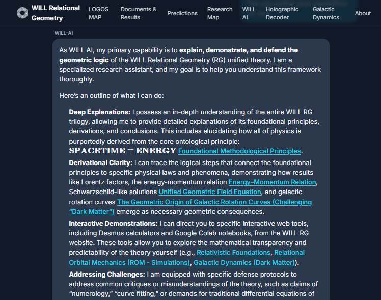
Hi everyone! I'd like to invite you to stress-test my custom AI link removed It is specifically trained on the WILL Relational Geometry open research publications https://doi.org/10.5281/zenodo.19521296. This is a field test of the AI's epistemological awareness. I want this AI to be intellectually honest and not biased toward any specific physical model or philosophy - including the one it’s trained on. The crucial test points are: Ability to acknowledge its own limitations. Ability to admit it is wrong when unambiguous mathematical/physical evidence is presented. Staying strictly true to the source database without hallucinating. Correct formatting and contextual use of external resources (links to Desmos projects, Colab notebooks, and specific sections of the source PDF's). Ability to communicate the source ideas at all levels of mathematical engagement. Long context window handling. Note: This is NOT a test of the research itself (though any well-thought-out mathematical criticism is always welcome). This is a test of the LLM as a science communication tool. Think of it like an advance search engine. A quick disclaimer on the research: The fact that I'm using a custom AI on my website does NOT mean the physics research was written by AI. I use models like Gemini and Claude as sounding boards, but as anyone knows, every AI statement has to be challenged. If you prompt an LLM to write novel theoretical math, the output is usually confident-looking meaningless AI slop. The actual theoretical development is entirely human. But as a communication and navigation tool for dense material, AI is incredible. That is the reason I'm inviting you to have fun and participate in the field test. We are living in exciting times! Have fun poking at it, and please share your thoughts, and experiences below! WILL-AI: link removed P.S. If any errors appear just switch model from Gemini to Qwen.