Kartazion
Senior Members
-
Joined
-
Last visited
Everything posted by Kartazion
-
 What do you think about that ? 'Minuscule traces' of virus in non-potable Paris water
 -
The problem also applies to the asymptomatic adult carriers. We'll have to test every one of us. As Many as 50 Percent of People with covid-19 Aren’t Aware They Have the Virus. See even Over 75% of people with covid-19 are asymptomatic.
-
That hidden viruses of the immunity could constitute a viral reservoir, and the immune defense no longer reach viruses. This viral reactivation is a possibility still under investigation.
-
This means that covid-19 can make a viral rebound and be reactivated in the case of a person who is already a carrier. The vaccine won't provide a solution if the virus is hiding. The vaccine will only be effective if the person has never had the virus, right? I found this in addition to info:
-
I had omitted that the term evolution was a specific stage reserved for the discipline of biology. I meant a database of immune memory that would be expanded and completed. I then discovered a strange organ because of its location in the body. The thymus. Here's what I could figure out. When the antigen is detected by the human body, it then produces lymphocytes ; B cells for antibodies, and T cells that destroy the infected cells. So why can't the immune system eradicate covid-19 in just a few moments? It's overwhelmed by the virus? Because the vaccine is giving the body time to prepare a sufficient number of antibodies? I hope I'm not off topic.
-
I meant to say making a synthetic antigen and injecting it into the patient so that his immune defense evolves. I see that it is very technical. Thank you again.
-
It was in 1930 in the United States that the first disease caused by a coronavirus was observed in poultry. It was in 1965 that the first coronavirus infecting humans (strain B814) was discovered. Act with the synthetic antigen to identify the virus in all its aspects? Will the immune response be effective in causing the production of special proteins for covid-19?
-
Thanks a lot for your answers. I concluded that these mutations, as numerous as they are, only very rarely result in a change in phenotype and viral function. In other words, the vaccine worked today will again be effective in 3 or 6 months.
-
Here is what I could read and understand about vaccines. The vaccine will depend on the mutation rate of the surface antigen (Spike protein). Protein S gathers in trimers on the surface of virions and plays a key role in the entry of the virus into its target cell. After the advanced protein binds to the human cell receptor, the viral membrane fuses with the human cell membrane, allowing the genome of the virus to enter human cells. We now detect three distinct variants of covid-19. Type A, B and C. I do not know if these mutations come from the S or L strains. Chinese researchers have also identified 149 minor variants among the 103 genomes analyzed. Indeed RNA viruses mutate much more easily and more quickly than DNA viruses, because with each replication, nucleic acids are poorly copied. My question is: The result of the mutation of the surface antigen is therefore more likely to degrade, than to succeed in a new link mechanism and membranes fusion, since they replicate poorly? I would even say that the virus is doomed to its loss. But I have also just seen that the purpose of mutating the virus is to overcome the resistance of the human immune system.
-
Do you think it can be done by accumulation and this in the long run? More longer we breathe it, more there will be in the body?
-
Yes indeed. And can we talk about a level of viral load and this in the air? Then we just need to know the threshold of the number of copies per millilitre to be infected. Or rather the number of copies inhaled per liter of air.
-
Ok. And I read this Coronavirus found in air samples from up to 13 feet from patients. Can we catch the virus from the air?
-
Here's some news about it. coronavirus-may-reactivate-in-cured-patients-korean-cdc-says
-
They are at unprecedented maximum plan The Italian government is not waiting. It is already fighting with all possible weapons. Clearly the Italian government does not let things go against the virus. If a vaccine arrives, then yes it will be welcome.
-
The exact words are: 'ça veut bien dire ce que ça veut dire' http://www.qalc.fr/question/expression-veut-bien-dire-elle-433796 The cleanest expression found in the dictionary is 'ça dit bien ce que ça veut dire' https://la-conjugaison.nouvelobs.com/definition/ca_dit_bien_ce_que_ca_veut_dire.php But let's not lose the essential. CharonY what do you think about this study, and what are the risks involved for us in everyday life?
-
In French we have an expression that says: 'ça veut dire ce que ça veut dire' Apparently it doesn't work with google translate Sorry about that.
-
Reuters wrote it like that: Coronavirus can persist in air for hours and on surfaces for days It means what it means.
-
Yes i'm also dumbfounded by this news. This is apparently the difference between SARS-CoV-2 compared to SARS-CoV-1. Here is the official publication with a little more info: https://www.nejm.org/doi/full/10.1056/NEJMc2004973 There is also a contact address
-
I think these minimum measures should be systematic. This poses a real problem when shopping at the supermarket. Here are the facts: Coronavirus lives for hours in air particles and days on surfaces
-
I do not know. Neither in immunity. CharonY will surely be able to answer us on this subject. But from what I heard, is that there is a case of recidivism at covid-19 in Japan; we can catch it a second time. Which brings up the question of knowing, and this because of chloroquine, would it not be for life in our body like paludism?
-
French doctrine is, in fact, not to test people with symptoms of the coronavirus, except for serious or complicated cases. In several weeks we will acquire some experience. So yes there will be a drastic protocol before you can operate in the professional field. For the moment our agents in France, whether they are police officers or nurses or workers, are not equipped. So I'll let you do the math.
-
Yes, but at what price? Phase 1: All essential businesses continue to operate. Phase 2: The working staff finds themselves sick. Phase 3: Shortage of the offer.
-
Just for confirmation: National Institutes of Health director: Up to 70K coronavirus cases could be confirmed in US by end of next week
-
The answer is most certainly yes. And this in all areas. Except for oil.
-
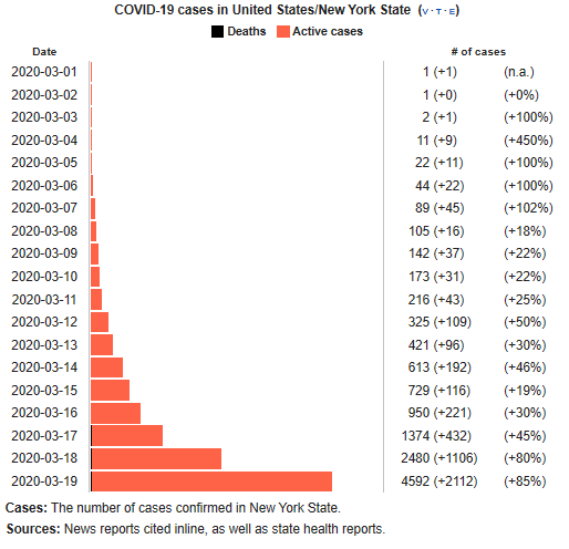
Corona virus are people just overeacting ? Now, no. Today, as of March 20, 2020, there are 14,366 cases of covid-19 in the United States. live of cases https://www.worldometers.info/coronavirus/country/us/ Americans must make the political decision adopted by China, Italy, France and Spain, and many other countries. Namely a complete confinement of residents to their homes. Without this, within a week the number of cases of covid-19 in the United States could be 70,000 people as of March 27, 2020. For another week, as of April 3, 2020, the number of cases would be 500,000 people. Between 2 and 3 million people by April 10, 2020. Several tens of millions within a full month. In France almost 34% of those infected are hospitalized, and around 10% are in intensive care. It is very likely that the rate of contamination in France, is largely underestimated. French doctrine is, in fact, not to test people with symptoms of the coronavirus, except for serious or complicated cases. Which would explain that. Fortunately there is already containment in the state of New York, but has reached an evolution of 80% per day this March 18 and 19. https://en.wikipedia.org/wiki/2020_coronavirus_pandemic_in_New_York_(state)