Mordred

The universe is smaller in the past when the photon gets emitted during its travel the universe expands how are you missing that detail ? the Universe is at its largest today and smaller in the past. Do you understand that part ? that is literally what expanding means

The blooming radius of the Observable universe pick any object or galaxy at the furthest you can examine and measure it how else do you think physics measures expansion pick any three or more galaxies and measure how they change distance from each other. I'm honestly beginning to feel your just trolling as no one an be that blind either that or you really need to study basic cosmology either that or I'm talking to some kid between ages 10 to 15. That has no prior knowledge of physics if thats true on the last part then we can help teach you the basics

the geometry is changing your photons must travel through spacetime. as the universe expands the distance your photons must travel increases. This leads to gravitational redshift which is Z. https://en.wikipedia.org/wiki/Gravitational_redshift That was the FLRW metric above the scale factor changes as your photons are trying to reach the observer. Here is the geometry again assume the flat case as its the easiest case \[d{s^2}=-{c^2}d{t^2}+a({t^2})[d{r^2}+{S,k}{(r)^2}d\Omega^2]\] \[S\kappa(r)= \begin{cases} R sin(r/R &(k=+1)\\ r &(k=0)\\ R sin(r/R) &(k=-1) \end {cases}\] if you want the line integral for flat the total interval along the Worldline (null geodesic photon path is) \[\delta S=\int^b_a=\sqrt{ds}=\int^b_a\sqrt{-cdt)^2+(dx)^2+(dy)^2+(dz)^2}\] so using the Radius of the universe and how it changes the distance becomes \[(dL)^2=(\frac{dr}{\sqrt{1-r^2}{/R^2}})^2+(r d\phi)^2\] so your photons must travel further the last 2 equations do not include scale factor changes but include the same relation to determine scale factor by \[a(t)\frac{r}{R}\]

How else do you think the scale factor is determined ? \[a(t)=\frac{R_{Then}}{R_{now}}\] so set radius of observable universe today as seen from Earth to 1 then determine what the scale factor is at a given Z using the equations of state. https://en.wikipedia.org/wiki/Equation_of_state_(cosmology) so if the Universe is half the volume at say z=1100 its not its just an example. then determine the scale factor using above relation. so here it is on a chart from z=1100 till today. \[{\scriptsize\begin{array}{|r|r|r|r|r|r|r|r|r|r|r|r|r|r|r|r|} \hline z&Scale (a)&T (Gyr)&R (Gly)&D_{now} (Gly)&D_{par}(Gly) \\ \hline 1.09e+3&9.17e-4&3.71e-4&6.25e-4&4.53e+1&8.38e-4\\ \hline 5.41e+2&1.84e-3&1.18e-3&1.91e-3&4.47e+1&2.78e-3\\ \hline 2.68e+2&3.71e-3&3.59e-3&5.64e-3&4.38e+1&8.88e-3\\ \hline 1.33e+2&7.47e-3&1.07e-2&1.64e-2&4.25e+1&2.75e-2\\ \hline 6.55e+1&1.50e-2&3.11e-2&4.73e-2&4.07e+1&8.32e-2\\ \hline 3.20e+1&3.03e-2&8.98e-2&1.36e-1&3.80e+1&2.47e-1\\ \hline 1.54e+1&6.09e-2&2.58e-1&3.89e-1&3.43e+1&7.27e-1\\ \hline 7.15e+0&1.23e-1&7.39e-1&1.11e+0&2.89e+1&2.12e+0\\ \hline 3.05e+0&2.47e-1&2.10e+0&3.12e+0&2.14e+1&6.13e+0\\ \hline 1.01e+0&4.97e-1&5.80e+0&8.05e+0&1.12e+1&1.74e+1\\ \hline 0.00e+0&1.00e+0&1.38e+1&1.45e+1&0.00e+0&4.62e+1\\ \hline \end{array}}\]

oh my so your telling me your lecturing me on how SR works with velocity which follows Galilean Relativity taught in high schools with the sole exception to the γ c and do not understand it applies to any NUMBER of observers INCLUDING 1 observer ? Your observer for example is at coordinate (ctx,y,z) apply those formulas I supplied above with velocity Use the distance to the horizon your length or radius of the Observable universe which is accelerating according to the Hubble's law formula I provided. The reason for the acceleration is due to the equations of state I mentioned. However it is also due to the length changing by an Natural logarithmic scale. All of those details are IN THE ARTICLE I posted. \[\acute{t}=\gamma(t-\frac{vc}{c^2})\] \[\acute{x}=\gamma(x-vt)\] then apply \[v_r=H_O d\] when you hit recessive velocity v=c the separation distance between observer to cosmological horizon will be zero \[ds^2=0\] That is true for all Observers who observe the recessive velocity when it reaches v=c using Hubble's law.

this is pointless quite frankly I'm reporting this thread for moderation. I'm done listening to garbage responses when its clear you cannot answer direct questions. What velocity are you applying to use the Lorentz transformations and where is your Length contraction which will reduce the separation distance to zero when v=c

if you ever do latex you need to edit to fix the latex. If your only applying simply one observer your examination is automatically wrong as any metric must be applicable for all observers.

Do you not know SR to even ask that ? Are you serious ? \[\acute{t}=\gamma(t-\frac{vc}{c^2})\] \[\acute{x}=\gamma(x-vt)\] Are you not familiar with this ? what velocity are you using to supply v to those equations?

try answering direct questions. what velocity are you using to apply the Lorentz transformation ? how are you factoring in length contraction ? or did you forget about length contraction ? which is part of the Lorentz transformations

There is no formula for cosmological time dilation not any SR based formula pure and simple. Cosmological time affinely connected to the scale factor under GR Newtonian weak field limit. If you read the article those formulas are contained within it. It clearly shows where precisely SR breaks down and also shows GR alone doesn't fully describe the FLRW metric. So don't ask for a formula that doesn't exist. \[d{s^2}=-{c^2}d{t^2}+a({t^2})[d{r^2}+{S,k}{(r)^2}d\Omega^2]\] \[S\kappa(r)= \begin{cases} R sin(r/R &(k=+1)\\ r &(k=0)\\ R sin(r/R) &(k=-1) \end {cases}\] proper time for commoving observers for cosmological time in the FLRW metric is this term \[-{c^2}d{t^2}\]

Your wasting ours if your here to state mainstream treatments are wrong and refuse to take the time to understand where your error lies when members show you the mainstream examinations. As you hit your 5 day limit I won't expect a reply till tomorrow. Take the time to read the article. Otherwise it's pointless for this thread to continue. If you cannot accept main stream physics responses then this thread If anything belongs in our Speculation forum and if you prefer attitude over learning will likely end up being locked.

No your not using msinstream physics nor mainstream SR so its pointless. Tell me what velocity are you using obviously your not applying recessive velocity \[v_{R}=H_oD\] in order to apply the lorentz transform so your not using SR let alone GR.

No offense but I have degrees in Cosmology it is my profession please listen to what is being described to you and read that link for starters. Secondly any member can participate regardless if whether you like the response or not. Your equation does not take into consideration the equations of state nor the acceleration equation of the FLRW metric. Your simulation doesn't match how our universe expands nor calculates it's expansion rate so comparison is incorrect. Still not enough range and the fact your twice the range tells me your doing SR in a non mainstream fashion ie not following the Lorentz transformations.

Won't have range using the above you will hit infinity at the Hubble horizon where recessive velocity exceeds c. This has been examined numerous times. One of the easier to understand examinations https://arxiv.org/abs/astro-ph/0310808

The error is not looking at the equations for time dilation nor looking at the distinction when the recessive velocity exceeds c. In cosmology cosmic time (proper time for commoving observers) follows the scale factor via an affine connection to the scale factor. Try looking at the equations of the FLRW metric which uses GR not some home brewed calculation. For starters you didn't mention to which Observer nor did you even mention the Lorentz transformations with the gamma factor nor the FLRW metric.

Vibration means any oscillating state. For example a spring in motion is a form of vibration. Sound waves generate vibrations. Fusion in Cosmology occurs during stsr formation but on a cosmological scale doesn't occur. The early atoms such as deuterium, hydrogen and lithium will form once temperatures cool down sufficiently. Now that Studiot went through the chemistry aspects let's try an example of why you need cooling. Take a proton it wants to have an electron in orbit due to charge. However the universe at high temperatures has tons of other particles moving about. So say the proton captures an electron. Now another particle comes along and knocks that electron out of orbit. The particle that does this is irrelevant. The only requirement is that it delivers enough force ( in energy equivalence 13.5 ev.) The above is an example of ionization. Cosmic rays can for example ionize neutral hydrogen in the same manner. If the Cosmic rays produce 13.5 ev the electron in the outer shell can get removed from the atom. In terms of fusion you require pressure and temperature. To reach ignition you must meet the Lawson criteria which will vary depending on the composition. https://en.m.wikipedia.org/wiki/Lawson_criterion Unfortunately most decent articles on nucleosythesis gets rather high level mathematics for example https://astro.uni-bonn.de/~nlanger/siu_web/nucscript/Nucleo.pdf But you will notice the article describes different binding energies for several different atoms.

I'm trying to get you to make the connection between the photon to E or B field. For example photons have no electric charge but has charge conjugation. So ask your self how do photons mediate electric charge ? If the photon never carries electric charge? It is the same direction Studiot is getting you to see and where the mathematics Swansont pointed out becomes essential

Every particle in the SM model has polarizations but those polarizations are not physical twists in space. Your adding effects not seen in any study of photons for example the known polarizations have physical effects when photons pass through a polarization filter yet yours do not. So why are your twists not seen in any experiment ? Also your mathematics do not include any wave vectors

Lol Though I never push personal favorite theories most my studies revolve around sterile neutrinos being a viable possibility. I do see a ton of lousy examinations of that possibility though. Part of attraction in that regards is that anti-neutrinos have never been detected though predicted by the models. That aside I find all the push of seeking "new physics" support articles rather annoying. I feel in those cases one should only look for "new physics " once all possibility of mainstream or current physics is clearly evident. I recall all the different Universe geometry papers prior to WMAP and Planck datasets the variations of possible geometries were staggering. So I tend to think of the current craze topic articles rather normal, as they've been around for pretty much any physics topic particularly when describing dynamics etc poorly understood or has a good body of clear evidence. Something that is oft overlooked in physics though is the mathematical developments finding ways to reduce computations of complex systems or finding means to organize all the possibilities such as through the use of gauge groups is oft never a big media blitz so you rarely hear of them. Yet they directly relate to development of fundamental physics . Too often it's the big media hits that get recognized rather than all the seemingly little discoveries or improved methodologies yet the little improvements could very well have a far greater range of applicability across other theories where they can be deployed.

While I agree with the comments above a couple other considerations in the past few decades several milestone advances have been reached. Examples being discovery of the Higgs boson this has the effect of causing a rather large paradigm shift. Detecting gravity waves Confirming neutrino mass Improved measurements of the CMB. Reduced number of possible geometries of the universe significantly. Those are just some examples in many ways were still catching up to those new available findings listed above.

good example of "beauty the beast" with that bite descriptive lol

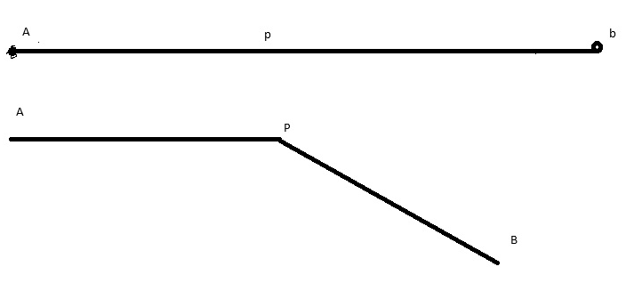
@DimaMazin I would like you to consider the following scenario now in the above signals sent by A and signals sent by B will be received at point P simultaneous as point P is the center between A and B. When you have a change in the magnitude component of velocity although you have length contraction this will not change. Treat this as 3 observers/emitters A,B,P However if that train goes around a corner which is also acceleration this is no longer true. If you were to draw a line between A and B Observer P will not fall on that line. It would not receive that signal. Instead P will only receive signals along the line from A to P and B to P but not the signal between A and B. So you are no longer dealing with one geodesic path of light but now three separate geodesic light paths. The geodesic path between A and B of the second case no longer goes through P but follows the hypotenuse connecting A and B If you were to say add another point in the second graph along the line connecting A and B and place another observer there. say Observer P_2. Then the events seen by P and P_2 observing A and B will not be seen simultaneous to each other by Observer P and P_2. This is a simple example where the notion of simultaneity breaks down. You have the same issue with curved spacetime. That issue is handled via rotations of the Lorentz transformations via a rotation matrix. Whereas is the first case change in magnitude of velocity it is a Boost not a rotation however in curved spacetime the light follows the curvature. These graphs ae simply a simple way to show the distinction between Lorentz transforms involving the two types of acceleration. A way to help understand why Proper time lies on a point of a geodesic path. That point is described by placing a tangent line to the surface of the curvature and have a parallel transported vector 90 degrees to that point connecting the Tangent vector to the curvature vector along with the perpendicular to the tangent connecting at the same point. Your convectors used under GR see figure 1.2 https://amslaurea.unibo.it/18755/1/Raychaudhuri.pdf figure 1.2 can be used to describe an Einstein train following a geodesic path not curvature of a physical object but rather the signal via photons. It show parallel transport along a geodesic path and the related mathematics that not only describe the observers but also how one can measure curvature using parallel transport which when you get down to is a form of train Einstein train PS In parallel transport the length connecting the parallel transported covectors is the affine connection in essence each section of the train following the geodesic please study the article and note how it leads ups to Principle of General Covariance: “The laws of physics in a general reference frame are obtained from the laws of Special Relativity by replacing tensor quantities of the Lorentz group with tensor quantities of the space-time manifold.”

Honestly I tried looking for extremely low order interactions, even the numerous graphs I looked through for any superconductor studies were well out of range. Consider this a single electron has greater energy than the value you just gave. The least massive SM particle with mass being neutrinos but the momentum term is still an issue In all honesty the best chance to get the idea working and not a terrible idea in and of itself is simply get rid of the 10^123 factor. Use the Bose-Einstein methodology would solve a great deal of the problem. It would be a very easy fix that way. Thst would go a long way back to feasible by just dropping that 10^123. Secondly use pions for the SU(3) atoms being the lightest meson and use the Maxwell boltzmann statistics to calculate number density. No confusion now you have a clear defined state to work from. That would also open up a large body of similar studies involving QCD Meissner. Epions actually require higher energy levels under SUSY so don't use a SUSY particle. If it were me those would be the route to address the issues.

Yeah your right good catch must have entered something wrong on calculator and didn't spot it. Too early in am last night. Still incredibly large energy density Well above current cosmological constant in joules/meter^3 for simplicity we can ignore spherical 10^45 ev/m^3 gives 1.60*10^26 joules/m^3

The authors unit is 10^-15 meters not meters^3 for range of force. Ie radius of each volume but just in case I will check them later after my meeting. It was 1 am when I did that set so will recheck