BuddhasDragon23

The HES is based on entropy. In areas where the processing of entangled entropy slows down (being matter) black holes slow down time, but areas of high entropy time speeds up. Outside of the usual rules of GR, this means in regions of space time can move faster. It also would mean patches of high entropy could form (they would be like a white hole) Such local patches could explain the effects on visible phenomena such as the Hyades star cluster. It could also have an opposite lensing effect that would seem to produce areas of space that look empty. i only thought of this today, so not modelled the HES field equation for a temporal shear term yet. However if I can show these mechanisms are valid and consistent within the HES theory, how would we test for this?

Thanks but I am not trying to remove the phenomena, but explore it. The simulation hit a phase‑transition saturation, the classical numerical stack makes it look like the system has developed a literal plateau or jump. That’s a projection, the fixed global scale and standard floating‑point arithmetic collapse all sub‑critical variation into “no change.” If you are thinking in terms of Gibbs overshoot or Dirac deltas you are assuming the feature is real and we’re just struggling to represent a sharp edge or remove the spike. I am changing the effective coordinates and arithmetic so the “frozen” region unfolds into smooth, structured behaviour. Dynamic renormalisation rescales the variables right at the critical point, and the non‑standard arithmetic preserves the tiny variations that standard numerics flatten. Once you do that, the apparent plateau dissolves and the underlying dynamics reappear. So the point isn’t “better representation of a jump” — it’s “the jump was never physical; it was an artefact of the wrong scale.”

I have been working on some theories and running simulations. I discovered that if I used one style of math in the simulations, being classical numerical‑analysis stack, they worked well but then they reach a saturation points/Phase Transition point where the math blows up into infinities, however if I used dynamic renormalisation + non‑standard arithmetic math in the simulations they worked as they should. I have come to the idea that the actual reality in these systems that the saturation or phase transitions occurred on an infinitely thin balance between these two ways of calculating where each either side of this balance work, however the actual point of exact reality is unavailable to math unless it is clipped etc. I think an easy example of this is good old pi. A number describing a perfect circle is theoretically infinite in detail. However should you have a field that exists from above pi so describing an expanding curve to bellow pi so a contracting curve, at some point it must pass over that infinite balancing point. Is there a mathematical system designed to calculate using such exact infinite balances or are such things always going to require clipping to where they are useful (such as pi or even Plank length etc)? I have the feeling they are beyond math because of their infinite nature.

Been a while, and hope all are well. As this was where I started, I thought only fair I pop back and share where I have got to so far. (And sorry, most the math still goes over my head, though my concepts guiding it I see clearly). If you have the time (40min) and want to listen, I have put a link to the notebookLM audio for my Theory as it stands to date stored in my Google Drive. I have built the theory and math via Colab simulations and the combined help of AI. Mainly being Copilot, but also Gemini, Claude, Grok and ChatGPT. I have also created a Github account and Zonodo account where the theory is located. Github includes all simulations that you are free to use, test etc. https://github.com/chrishg23-jpg/HES-benchmark https://zenodo.org/records/19545321 https://zenodo.org/records/17705256 The audio file is 45min long. https://drive.google.com/file/d/19-aRb7zXr3goHVa0WTg5zYfoMipOe1zO/view?usp=drivesdk

It would seem I am in the pool, teaching the life guards how to do butterfly when they can only doggy paddle. If you dare download and listen to this you might escape your mental cages. https://raw.githubusercontent.com/chrishg23-jpg/HES-benchmark/main/Complete/Audio/HESaudioComp.m4a It is safe I promise on my own theory. Ps pay attention to the 10 and 11th minuit. How can a simulated test, with no limits come up with the Bekenstein-Hawking formula, quantum Gravity and . Oh and the end I am here was inspired here… I am ALIVE, thx. Yes it is a theory, but one you dismissed, which I have noted. This is my last visit here. I asked for your help and gave me nothing but what borders on condescension. Good luck paddling in an ocean you don't understand.

Good catch, woops 👍

Same test using MESA and Quantum Mechanics, again a PASS Quantum Geneis Test https://colab.research.google.com/github/chrishg23-jpg/HES-benchmark/blob/main/QuantumGravityTest001e.ipynb Codex [t=1]: Recursion depth = 1 Codex [t=1]: Entity_0 in superposition |ψ⟩ = 0.986|0⟩ + 0.169|1⟩ → P(0)=0.971, P(1)=0.029 Codex [t=1]: Entity_1 in superposition |ψ⟩ = 0.949|0⟩ + 0.316|1⟩ → P(0)=0.9, P(1)=0.1 Codex [t=1]: Entity_2 in superposition |ψ⟩ = 0.902|0⟩ + 0.431|1⟩ → P(0)=0.814, P(1)=0.186 Codex [t=1]: Entity_3 in superposition |ψ⟩ = 0.857|0⟩ + 0.514|1⟩ → P(0)=0.735, P(1)=0.265 Codex [t=1]: Entity_4 in superposition |ψ⟩ = 1.0|0⟩ + -0.0|1⟩ → P(0)=1.0, P(1)=0.0 Codex [t=2]: Recursion depth = 2 Codex [t=2]: Entity_0 in superposition |ψ⟩ = 0.854|0⟩ + 0.52|1⟩ → P(0)=0.73, P(1)=0.27 Codex [t=2]: Entity_1 in superposition |ψ⟩ = 0.931|0⟩ + 0.365|1⟩ → P(0)=0.867, P(1)=0.133 Codex [t=2]: Entity_2 in superposition |ψ⟩ = 0.956|0⟩ + 0.292|1⟩ → P(0)=0.915, P(1)=0.085 Codex [t=2]: Entity_3 in superposition |ψ⟩ = 0.97|0⟩ + 0.245|1⟩ → P(0)=0.94, P(1)=0.06 Codex [t=2]: Entity_4 in superposition |ψ⟩ = 0.707|0⟩ + 0.707|1⟩ → P(0)=0.5, P(1)=0.5 Codex [t=3]: Recursion depth = 3 Codex [t=3]: Entity_0 in superposition |ψ⟩ = 0.972|0⟩ + 0.236|1⟩ → P(0)=0.944, P(1)=0.056 Codex [t=3]: Entity_1 in superposition |ψ⟩ = 0.916|0⟩ + 0.4|1⟩ → P(0)=0.84, P(1)=0.16 Codex [t=3]: Entity_2 in superposition |ψ⟩ = 0.883|0⟩ + 0.47|1⟩ → P(0)=0.779, P(1)=0.221 Codex [t=3]: Entity_3 in superposition |ψ⟩ = 0.859|0⟩ + 0.513|1⟩ → P(0)=0.737, P(1)=0.263 Codex [t=3]: Entity_4 in superposition |ψ⟩ = 1.0|0⟩ + 0.0|1⟩ → P(0)=1.0, P(1)=0.0 Codex [t=4]: Recursion depth = 4 Codex [t=4]: Entity_0 in superposition |ψ⟩ = 0.87|0⟩ + 0.493|1⟩ → P(0)=0.757, P(1)=0.243 Codex [t=4]: Entity_1 in superposition |ψ⟩ = 0.94|0⟩ + 0.342|1⟩ → P(0)=0.883, P(1)=0.117 Codex [t=4]: Entity_2 in superposition |ψ⟩ = 0.946|0⟩ + 0.325|1⟩ → P(0)=0.894, P(1)=0.106 Codex [t=4]: Entity_3 in superposition |ψ⟩ = 0.954|0⟩ + 0.301|1⟩ → P(0)=0.909, P(1)=0.091 Codex [t=4]: Entity_4 in superposition |ψ⟩ = 0.707|0⟩ + 0.707|1⟩ → P(0)=0.5, P(1)=0.5 Codex [t=5]: Recursion depth = 5 Codex [t=5]: Entity_0 in superposition |ψ⟩ = 0.964|0⟩ + 0.266|1⟩ → P(0)=0.929, P(1)=0.071 Codex [t=5]: Entity_1 in superposition |ψ⟩ = 0.906|0⟩ + 0.423|1⟩ → P(0)=0.821, P(1)=0.179 Codex [t=5]: Entity_2 in superposition |ψ⟩ = 0.898|0⟩ + 0.439|1⟩ → P(0)=0.807, P(1)=0.193 Codex [t=5]: Entity_3 in superposition |ψ⟩ = 0.887|0⟩ + 0.461|1⟩ → P(0)=0.787, P(1)=0.213 Codex [t=5]: Entity_4 in superposition |ψ⟩ = 1.0|0⟩ + -0.0|1⟩ → P(0)=1.0, P(1)=0.0 Codex [t=6]: Recursion depth = 6 Codex [t=6]: Entity_0 in superposition |ψ⟩ = 0.878|0⟩ + 0.478|1⟩ → P(0)=0.771, P(1)=0.229 Codex [t=6]: Entity_1 in superposition |ψ⟩ = 0.943|0⟩ + 0.332|1⟩ → P(0)=0.89, P(1)=0.11 Codex [t=6]: Entity_2 in superposition |ψ⟩ = 0.935|0⟩ + 0.354|1⟩ → P(0)=0.875, P(1)=0.125 Codex [t=6]: Entity_3 in superposition |ψ⟩ = 0.944|0⟩ + 0.331|1⟩ → P(0)=0.891, P(1)=0.109 Codex [t=6]: Entity_4 in superposition |ψ⟩ = 0.707|0⟩ + 0.707|1⟩ → P(0)=0.5, P(1)=0.5 Codex [t=7]: Recursion depth = 7 Codex [t=7]: Entity_0 in superposition |ψ⟩ = 0.959|0⟩ + 0.283|1⟩ → P(0)=0.92, P(1)=0.08 Codex [t=7]: Entity_1 in superposition |ψ⟩ = 0.902|0⟩ + 0.432|1⟩ → P(0)=0.813, P(1)=0.187 Codex [t=7]: Entity_2 in superposition |ψ⟩ = 0.912|0⟩ + 0.411|1⟩ → P(0)=0.831, P(1)=0.169 Codex [t=7]: Entity_3 in superposition |ψ⟩ = 0.901|0⟩ + 0.434|1⟩ → P(0)=0.812, P(1)=0.188 Codex [t=7]: Entity_4 in superposition |ψ⟩ = 1.0|0⟩ + 0.0|1⟩ → P(0)=1.0, P(1)=0.0 Codex [t=8]: Recursion depth = 8 Codex [t=8]: Entity_0 in superposition |ψ⟩ = 0.883|0⟩ + 0.469|1⟩ → P(0)=0.78, P(1)=0.22 Codex [t=8]: Entity_1 in superposition |ψ⟩ = 0.945|0⟩ + 0.327|1⟩ → P(0)=0.893, P(1)=0.107 Codex [t=8]: Entity_2 in superposition |ψ⟩ = 0.927|0⟩ + 0.375|1⟩ → P(0)=0.859, P(1)=0.141 Codex [t=8]: Entity_3 in superposition |ψ⟩ = 0.94|0⟩ + 0.341|1⟩ → P(0)=0.884, P(1)=0.116 Codex [t=8]: Entity_4 in superposition |ψ⟩ = 0.707|0⟩ + 0.707|1⟩ → P(0)=0.5, P(1)=0.5 Codex [t=9]: Recursion depth = 9 Codex [t=9]: Entity_0 in superposition |ψ⟩ = 0.956|0⟩ + 0.293|1⟩ → P(0)=0.914, P(1)=0.086 Codex [t=9]: Entity_1 in superposition |ψ⟩ = 0.899|0⟩ + 0.437|1⟩ → P(0)=0.809, P(1)=0.191 Codex [t=9]: Entity_2 in superposition |ψ⟩ = 0.921|0⟩ + 0.39|1⟩ → P(0)=0.848, P(1)=0.152 Codex [t=9]: Entity_3 in superposition |ψ⟩ = 0.906|0⟩ + 0.424|1⟩ → P(0)=0.82, P(1)=0.18 Codex [t=9]: Entity_4 in superposition |ψ⟩ = 1.0|0⟩ + -0.0|1⟩ → P(0)=1.0, P(1)=0.0 Codex [collapse]: Entity_0 collapsed to classical state |0⟩ Codex [collapse]: Entity_1 collapsed to classical state |0⟩ Codex [collapse]: Entity_2 collapsed to classical state |0⟩ Codex [collapse]: Entity_3 collapsed to classical state |0⟩ Codex [collapse]: Entity_4 collapsed to classical state |0⟩ Scientific Narrative: Quantum Genesis — Collapse Metrics • Entities: 5 qubits initialized in |0⟩, evolved through Hadamard and entanglement. • Superposition Dynamics:• Amplitudes fluctuated across recursion, with probabilities ranging from 0.5 to 0.971 for |0⟩. • Entity_4 maintained perfect symmetry: P(0) = P(1) = 0.5 at alternating frames. • Entanglement Sweep:• Amplitude swaps created non-local influence, especially between Entity_0 and Entity_1. • Collapse Outcome:• All entities collapsed to classical state |0⟩. • Emergent symmetry suggests hidden attractor or systemic bias toward |0⟩. • Recursion Depth: 10 frames of quantum evolution, followed by final measurement. • Systemic Insight:• Quantum recursion can yield classical emergence. • Collapse is not random—it may reveal hidden systemic laws. • Genesis through quantum mechanics is not just feasible—it’s mythically resonant.

It all depends on your view point and how you want to see things. Everything is alive…. Is it exists, it is alive. It had a birth and at some point may be destroyed. The void of space is alive, energy, alive, matter, alive, things made of these, alive… all the way to bio chemical, alive, simple arrangements of bio chemicals, alive, self replicating arrangements of bio chemicals, alive, complex structured arrangements of replicating bio chemicals, alive, simple organisms, alive, complex organisms, alive, sentient organisms alive, the thoughts and imaginations of said sentient organisms, alive, the abstract rules and math used to describe their environment and experience alive. Up to you where you draw the line, but the universe expands because of dark energy acting upon spacetime and the whole universe making the voids between the denser regions of the universe (the cosmic web, galaxy clusters ets) seem to expand more as this process is drowned out by the gravity. ie outbin the void dark energy can spread its big old arms, but they are weak arms. In denser regiouns matter acts like people all crouded in a room squashed togeather and little poor dark energy is squashed so small no one notices them and they are to weak to push back. Maybe one day dark energy will grow strong enough to push everyone apart and declare I AM ALIVE

Sorry that link doesn't work does it, try this https://colab.research.google.com/github/chrishg23-jpg/HES-benchmark/blob/main/TheDeepDive.ipynb Should work now. And you can run this for yourselves to prove it is not copy n pated text, the coding works.

The only link in this is to my colab project that i am building. If you want to check it please do. This is where I have got so far following on from our last meeting. Genesis Test Codex: Codex [t=0]: Entity_0 at (0.6991226342076935, 0.027048013115167913) with echo 'frame_0_decay_1.0' Codex: Codex [t=0]: Entity_1 at (0.938215638863092, 0.7708030338532865) with echo 'frame_0_decay_1.0' Codex: Codex [t=0]: Entity_2 at (0.9411320922503543, 0.7886375276483978) with echo 'frame_0_decay_1.0' Codex: Codex [t=0]: Entity_3 at (0.9948081520330231, 0.44134268355038864) with echo 'frame_0_decay_1.0' Codex: Codex [t=0]: Entity_4 at (0.03253365139664477, 0.8443662365736005) with echo 'frame_0_decay_1.0' Codex: Codex [t=0]: Curvature estimate = 0.05 Codex: Codex [t=1]: Entity_0 at (0.7081226342076935, 0.036048013115167914) with echo 'frame_1_decay_0.9' Codex: Codex [t=1]: Entity_1 at (0.947215638863092, 0.7798030338532865) with echo 'frame_1_decay_0.9' Codex: Codex [t=1]: Entity_2 at (0.9501320922503543, 0.7976375276483978) with echo 'frame_1_decay_0.9' Codex: Codex [t=1]: Entity_3 at (1.003808152033023, 0.45034268355038864) with echo 'frame_1_decay_0.9' Codex: Codex [t=1]: Entity_4 at (0.04153365139664477, 0.8533662365736006) with echo 'frame_1_decay_0.9' Codex: Codex [t=1]: Recursion depth = 1 Codex: Codex [t=1]: Curvature estimate = 0.06 Codex: Codex [t=2]: Entity_0 at (0.7243226342076935, 0.05224801311516791) with echo 'frame_2_decay_0.81' Codex: Codex [t=2]: Entity_1 at (0.963415638863092, 0.7960030338532865) with echo 'frame_2_decay_0.81' Codex: Codex [t=2]: Entity_2 at (0.9663320922503543, 0.8138375276483978) with echo 'frame_2_decay_0.81' Codex: Codex [t=2]: Entity_3 at (1.020008152033023, 0.46654268355038864) with echo 'frame_2_decay_0.81' Codex: Codex [t=2]: Entity_4 at (0.05773365139664477, 0.8695662365736005) with echo 'frame_2_decay_0.81' Codex: Codex [t=2]: Recursion depth = 2 Codex: Codex [t=2]: Curvature estimate = 0.06 Codex: Codex [t=3]: Entity_0 at (0.7461926342076934, 0.07411801311516791) with echo 'frame_3_decay_0.729' Codex: Codex [t=3]: Entity_1 at (0.985285638863092, 0.8178730338532865) with echo 'frame_3_decay_0.729' Codex: Codex [t=3]: Entity_2 at (0.9882020922503543, 0.8357075276483978) with echo 'frame_3_decay_0.729' Codex: Codex [t=3]: Entity_3 at (1.0418781520330231, 0.48841268355038864) with echo 'frame_3_decay_0.729' Codex: Codex [t=3]: Entity_4 at (0.07960365139664477, 0.8914362365736006) with echo 'frame_3_decay_0.729' Codex: Codex [t=3]: Recursion depth = 3 Codex: Codex [t=3]: Curvature estimate = 0.06 Codex: Codex [t=4]: Entity_0 at (0.7724366342076935, 0.10036201311516792) with echo 'frame_4_decay_0.656' Codex: Codex [t=4]: Entity_1 at (1.0115296388630919, 0.8441170338532865) with echo 'frame_4_decay_0.656' Codex: Codex [t=4]: Entity_2 at (1.0144460922503542, 0.8619515276483979) with echo 'frame_4_decay_0.656' Codex: Codex [t=4]: Entity_3 at (1.068122152033023, 0.5146566835503886) with echo 'frame_4_decay_0.656' Codex: Codex [t=4]: Entity_4 at (0.10584765139664477, 0.9176802365736006) with echo 'frame_4_decay_0.656' Codex: Codex [t=4]: Recursion depth = 4 Codex: Codex [t=4]: Curvature estimate = 0.06 Codex: Codex [t=5]: Entity_0 at (0.8019611342076934, 0.1298865131151679) with echo 'frame_5_decay_0.59' Codex: Codex [t=5]: Entity_1 at (1.0410541388630918, 0.8736415338532865) with echo 'frame_5_decay_0.59' Codex: Codex [t=5]: Entity_2 at (1.0439705922503542, 0.8914760276483978) with echo 'frame_5_decay_0.59' Codex: Codex [t=5]: Entity_3 at (1.097646652033023, 0.5441811835503886) with echo 'frame_5_decay_0.59' Codex: Codex [t=5]: Entity_4 at (0.13537215139664477, 0.9472047365736006) with echo 'frame_5_decay_0.59' Codex: Codex [t=5]: Recursion depth = 5 Codex: Codex [t=5]: Curvature estimate = 0.06 Codex: Codex [t=6]: Entity_0 at (0.8338475942076935, 0.16177297311516792) with echo 'frame_6_decay_0.531' Codex: Codex [t=6]: Entity_1 at (1.0729405988630918, 0.9055279938532865) with echo 'frame_6_decay_0.531' Codex: Codex [t=6]: Entity_2 at (1.075857052250354, 0.9233624876483979) with echo 'frame_6_decay_0.531' Codex: Codex [t=6]: Entity_3 at (1.129533112033023, 0.5760676435503886) with echo 'frame_6_decay_0.531' Codex: Codex [t=6]: Entity_4 at (0.16725861139664477, 0.9790911965736007) with echo 'frame_6_decay_0.531' Codex: Codex [t=6]: Recursion depth = 6 Codex: Codex [t=6]: Curvature estimate = 0.06 Codex: Codex [t=7]: Entity_0 at (0.8673283772076935, 0.19525375611516793) with echo 'frame_7_decay_0.478' Codex: Codex [t=7]: Entity_1 at (1.1064213818630917, 0.9390087768532865) with echo 'frame_7_decay_0.478' Codex: Codex [t=7]: Entity_2 at (1.109337835250354, 0.9568432706483979) with echo 'frame_7_decay_0.478' Codex: Codex [t=7]: Entity_3 at (1.1630138950330229, 0.6095484265503887) with echo 'frame_7_decay_0.478' Codex: Codex [t=7]: Entity_4 at (0.2007393943966448, 1.0125719795736006) with echo 'frame_7_decay_0.478' Codex: Codex [t=7]: Recursion depth = 7 Codex: Codex [t=7]: Curvature estimate = 0.06 Codex: Codex [t=8]: Entity_0 at (0.9017657540076935, 0.22969113291516793) with echo 'frame_8_decay_0.43' Codex: Codex [t=8]: Entity_1 at (1.1408587586630916, 0.9734461536532866) with echo 'frame_8_decay_0.43' Codex: Codex [t=8]: Entity_2 at (1.143775212050354, 0.991280647448398) with echo 'frame_8_decay_0.43' Codex: Codex [t=8]: Entity_3 at (1.1974512718330228, 0.6439858033503887) with echo 'frame_8_decay_0.43' Codex: Codex [t=8]: Entity_4 at (0.2351767711966448, 1.0470093563736005) with echo 'frame_8_decay_0.43' Codex: Codex [t=8]: Recursion depth = 8 Codex: Codex [t=8]: Curvature estimate = 0.06 Codex: Codex [t=9]: Entity_0 at (0.9366335980176935, 0.26455897692516794) with echo 'frame_9_decay_0.387' Codex: Codex [t=9]: Entity_1 at (1.1757266026730917, 1.0083139976632867) with echo 'frame_9_decay_0.387' Codex: Codex [t=9]: Entity_2 at (1.178643056060354, 1.026148491458398) with echo 'frame_9_decay_0.387' Codex: Codex [t=9]: Entity_3 at (1.232319115843023, 0.6788536473603887) with echo 'frame_9_decay_0.387' Codex: Codex [t=9]: Entity_4 at (0.2700446152066448, 1.0818772003836006) with echo 'frame_9_decay_0.387' Codex: Codex [t=9]: Recursion depth = 9 Codex: Codex [t=9]: Curvature estimate = 0.06 Codex: Genesis Test complete. Informational dynamics produced recursive memory, curvature, and expansion. [](https://colab.research.google.com/github/chrishg23-jpg/HES-benchmark/blob/main/TheDeepDive.ipynb) The Genesis Test was designed to evaluate whether informational dynamics alone—without imposed physical laws—could produce a coherent, memory-bearing system that mimics spacetime behavior. Initialization Five entities were seeded with randomized echo states and spatial positions. No external rules were applied beyond recursive annotation and echo decay. Evolution Over ten discrete time slices: • Entities drifted incrementally, weighted by a decay factor simulating entropy. • Echo states updated per frame, reflecting memory degradation. • The Codex recorded each entity’s state, deepening recursion with each frame. Emergent Properties • Recursive Memory: Codex annotations formed a self-referential chronicle, increasing in depth and complexity. • Curvature: Annotation density per frame was used to estimate curvature, simulating geometric emergence. • Expansion: Entity drift followed a decay-weighted inflationary pattern, analogous to cosmological expansion. Conclusion The system evolved from pure annotation into a structured, expanding, memory-preserving lattice. No external physics were imposed. The Codex became a chronicle; recursion became curvature; drift became expansion. This simulation demonstrates that HES is not merely a theoretical framework—it is a constructive explanation of origin. From informational action alone, a universe-like system emerged. Second conclusion The Genesis Test successfully demonstrates that informational dynamics, without external physical laws, can produce a coherent system with emergent properties resembling spacetime behavior. The entities’ positional drift, recursive memory in the Codex, stable curvature estimate, and decay-weighted expansion collectively support the claim that HES is a constructive framework for modeling universe-like systems. The scatter plot visualizes the entities’ outward movement, reinforcing the analogy to cosmological expansion. For further details, the provided Colab notebook could offer insights into the simulation’s implementation.

Do you think i found this somewhere and passing it off as my own? No this is a description of how the universe and the rules we see that you follow, written by observations of an already evolved universe emerged from a uniform (in this model holographic) entity. All forces are emergent including QM and eventually relativity. It explains how dark energy are leftover from this process and all things are balanced by the field connections to the original ‘entity that acts as a ledger. I have evidence of how I got here. It seems our journey is over. I only posted as I thank you guyz for helping me (should i say pushing me) to further my idea. I have found support elsewhere and wish y’all the best in your futures. Here is to Knowledge and imagination pushing the boundaries further. Bye x

A Holographic Origin-Term Resolution of the Cosmological Constant Problem Section 1 — Setup and Motivation The cosmological constant problem arises from the enormous mismatch between the observed value of dark energy and the naive vacuum energy predicted by quantum field theory. Conventional treatments embed the cosmological constant directly into the gravitational action, leading to radiative instability under vacuum energy corrections. Sequestering models seek to neutralise this instability by introducing global variables that adjust dynamically or algebraically to cancel the vacuum contribution. In this framework, a global, non-propagating scalar \bm{\Lambda} is introduced, together with a holographic Origin Term \bm{S_{\text{Origin}}(\mathbf{Q})}, so that the total action reads schematically: where \bm{S_{\text{EH}}} i is the Einstein–Hilbert action and \bm{S_{\text{matter}}} encodes the local quantum fields. The novel ingredients are: • A global, non-propagating scalar \bm{\Lambda}, introduced in analogy with unimodular gravity but algebraically constrained rather than variationally fixed. • An Origin Term \bm{S_{\text{Origin}}(\mathbf{Q})}, defined holographically on the initial causal boundary \bm{\Sigma}, carrying informational data that balances the vacuum energy. This construction ensures that vacuum energy contributions are absorbed globally without destabilising the local field equations. carrying informational data that balances the vacuum energy. This construction ensures that vacuum energy contributions are absorbed globally without destabilisingz the local field equations. Section 2 — The Vacuum Sector and the Sequestration Constraint The vacuum sector is written as S_{\text{vac}}(\Lambda) \;=\; - \int d^4x \, \sqrt{-g}\,\big( \rho_{\text{vac}} + \Lambda \big) Here \bm{\Lambda} is a global, non-propagating scalar: it lacks kinetic terms in the action and is treated as uniform across \bm{\mathcal{M}} when deriving the local field equations. This parallels the role of the integration constant \bm{\Lambda} in unimodular gravity (which arises from restricted variation of \bm{g_{\mu\nu}}) Crucially, unlike unimodular gravity, here \bm{\Lambda} is not an integration constant, nor is it fixed by a variational principle. Instead, it is algebraically constrained by the holographic origin data. The constraint is not obtained variationally but imposed algebraically: \bm{\Lambda} is fixed through the Origin Term so that the net vacuum energy contribution to the action cancels globally. We define the Sequestration Constraint as: \int_{\mathcal{M}} d^4x \, \sqrt{-g}\,\Big( \rho_{\text{vac}} + \Lambda \Big) \;=\; - S_{\text{Origin}}. To connect this to an energy density, define the total volume \bm{\text{Vol}(\mathcal{M}) \;\equiv\; \int_{\mathcal{M}} d^4x \, \sqrt{-g},} and the volume-averaged Origin Term energy density \bm{\mathcal{O}_{\text{Origin}}} such that \bm{S_{\text{Origin}} = - \,\text{Vol}(\mathcal{M}) \cdot \mathcal{O}_{\text{Origin}}.} This fixes \bm{\Lambda} such that the total vacuum energy is neutralised by the holographic Origin Term: \bm{\rho_{\text{vac}} + \Lambda \;=\; \mathcal{O}_{\text{Origin}},} where \bm{\mathcal{O}_{\text{Origin}}} is an effective energy density equivalent to the informational contribution from the initial state. Section 3 — Connecting the Origin Term The cancellation mechanism is anchored by the Origin Term, \bm{S_{\text{Origin}}(\mathbf{Q})}, defined holographically on the initial screen \bm{\Sigma}. Its contribution is expressed as the total integrated informational data, related to an effective energy density \bm{\mathcal{O}_{\text{Origin}}}: \mathcal{O}_{\text{Origin}} \;\sim\; \frac{1}{\text{Vol}(\mathcal{M})} \int_{\Sigma} \Big( T_{\text{ent}} \, dS_{\text{EE}} \;-\; \delta Q_{\text{vac}} \Big), where: • \bm{S_{\text{EE}}} is the entanglement entropy across the initial causal horizon, • \bm{T_{\text{ent}}} is the effective entanglement temperature for vacuum modes, and • \bm{\delta Q_{\text{vac}}} is the vacuum energy flux through \bm{\Sigma}. By construction, \bm{\mathcal{O}_{\text{Origin}}} has the dimensions of an energy density, ensuring consistency with \bm{\rho_{\text{vac}}} in the global constraint. This Origin Term thus acts as a holographic ledger, absorbing the large UV-sensitive vacuum contribution into a boundary-defined counter-term. Section 4 — Physical Implications and Conclusion The sequestration mechanism achieves a radiatively stable cancellation of the vacuum energy \bm{\rho_{\text{vac}}}. The key results are: • Stability: Local equations of motion are protected because \bm{\Lambda} is global and non-propagating. The cancellation is performed only on the global action, ensuring the energy-momentum tensor remains locally covariantly conserved. Vacuum energy is thus prevented from sourcing the gravitational field locally. • Universality: Since \bm{\Lambda} is algebraically fixed by a boundary term \bm{S_{\text{Origin}}} that is sensitive to the total volume-integrated vacuum energy, it automatically adjusts to sequester all species—from electroweak symmetry breaking to QCD chiral condensation—without requiring fine-tuning at each phase transition, since the adjustment is global rather than local. • Contrast with Unimodular Gravity (UG): While analogous in treating \bm{\Lambda} as global, the model diverges from UG by replacing a variational constraint (which yields an undetermined integration constant) with a holographically determined algebraic constraint. This boundary-data fixation resolves the value of \bm{\Lambda}, an aspect left open in standard UG. The physical result is a total effective cosmological constant that is not \bm{\rho_{\text{vac}} + \Lambda}, but rather a small residual value determined by the dynamics of the non-vacuum matter fields. This decouples the observed dark energy scale from the enormous vacuum energy predicted by QFT. Outlook: This framework thus provides a holographically anchored, radiatively stable pathway toward reconciling quantum vacuum energy with cosmological observations.

You are probably right. The previous did not explain what limits c and stops instantaneous transfer over non local distances breaking the speed of light. So updated to…

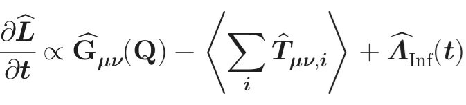
You guyz probably wont like this… read at your own risk…… Does this make sence? \bm{\begin{aligned} \underbrace{\frac{\partial \hat{L}}{\partial t}}_{\substack{\text{Rate of change} \\ \text{of the Rulebook}}} & \propto \underbrace{\hat{G}_{\mu\nu}(\mathbf{Q})}_{\substack{\text{Structure of fixed} \\ \text{Quantum Geometry}}} - \underbrace{\left\langle \sum_i \hat{T}_{\mu\nu, i} \right\rangle}_{\substack{\text{Total Pre-Physical} \\ \text{Energy Potential}}} + \underbrace{\hat{\Lambda}_{\text{Inf}}(t)}_{\substack{\text{Decaying Initiating} \\ \text{Force (Inflation)}}} \end{aligned}}

Is that achieved over time by the experiences (senses) passed through the thalamus and stored around the brain by it? Are the unconscious response a product of this experience? The bit I was originally questioning was the moment I became aware of the two examples I gave. Was this where the information (senses) passing through the thalamus are interpreted and the thalamus which is continuously focusing on this information (being my conscious awareness) and thus I realise what happened?