Schindelbeck

If anyone wants some more detailed information, they can find it here: kaluza-without-klein.net/short.pdf Happy holidays!

c_0 in flat spacetime (4D). Otherwise I think there is no sharp boundary. In curved space-time you’ll have light deflection, Shapiro delay. Since photons themselves contribute to the curvature, there might be a possibility for self-trapping. With the modified Kaluza model the orders of magnitude will match particle energies.

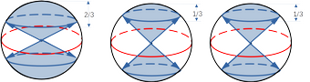
I’ll give part II a try: The Kaluza model with spin 1/2 as boundary condition described above has a corresponding, related toy model for particles: A circular polarized photon with its intrinsic angular momentum interpreted as having its E- and B-vectors rotating around a central axis of propagation will be transformed into an object that has the - still rotating - E-vector constantly oriented to a fixed point , the origin of a local coordinate system. The vectors E, B and C of the propagation velocity are supposed to be locally orthogonal and originating at a common point, the center of rotation (the C-vector will take part in the rotation). This has the following qualitative consequences: 1) Such a rotation is related to the group SO(3) (and SU(2) as important special case). 2) E-vector constantly oriented to a fixed point implies charge. 3) A local coordinate system = rest system implies mass. 4) In case of any lateral extension of the E-field, for r -> 0 the overlap of a rotating E-vector implies rising energy density, resulting in rising curvature of space-time (which will be the mechanism for such a self-trapping – quantiatively described by the Kaluza ansatz of the 1st post) 5) The orthogonal vectors E, B and C can be given in 2 different chiral states (left- right-handed). 6) As waves such states are consistent with a “point-like” structure function on the other hand imply a spatial distribution of energy density and angular momentum / spin. That’s a pretty simple toy model, but we are talking about electric and magnetic fields. You can calculate them (their relative values). For quantitative results 3 orthonormal vectors E, B, C, each described as imaginary part of a quaternion with real part 0, will be subject to alternate, incremental rotations around the axes E, B and C. Only solutions where one of the incremental angles of rotation has half the value of the other two will be considered. This may serve as a primitive model for spin J=1/2. There are 3 possible solutions corresponding to half the angular frequency for each of the components E, B, or C, each giving a trajectory where the E-vector encloses a spherical cone. The spherical cap of the cone encompasses a fraction of the area of a hemisphere of 2/3, 1/3 and 1/3, respectively (see fig. below). Mirroring at the center of rotation gives the equivalent double cone (blue), the fractions of both caps in relation to the surface of the total sphere may be interpreted to give partial charges of 2/3, 1/3 and 1/3 according to Gauss’ law. It is suggestive to identify such components with analogues of UDS-quarks. The E-vector might as well be interpreted to enclose the complement of the double cone of a 3D-ball (white), a spherical wedge. This gives the objects complement-U, complement-D, complement-S attributable to charges 1/3, 2/3, 2/3. These objects may be attributed to c, b, t-quarks. Such UDSCBT-entities of (single) spherical cones and toroidal wedges may be used as elementary building blocks to be combined to form more complex objects pending on fitting phase / angular momentum and chirality as well as interference of the fields itself. A mismatch in phase/ chirality may result in nodal planes and higher energy states. It will be left undecided, if more complex compositions of such objects might be interpreted to represent time averages of propagating EBC-vectors or a standing wave. The simplest objects will result from combining an U, D or S-component with its complement of same phase and chirality, which formally will reassemble the complete sphere. These objects may be attributed to the charged and neutral* leptons (*Implying the center of rotation is not at the “tip” of an E-vector, but at its “center”). An electron might be considered e.g. as an (anti-U + (U-Complement = B)) particle, however, unlike a B-meson with spin 1/2. While this is not possible with quarks, i.e. objects with particle character, it is possible with an electromagnetic wave. (Side note on neutrinos: they are a little special in this model. However, if you extend the series of particle energies below the electron with the next power of alpha, i.e. [math]\alpha^9[/math] you will be in the range of 0.1eV which is the expected range for neutrino energy.) An even more sensitive test is the calculation of magnetic moments of uds-baryons. I can give only a sketch. A combination of 3 orthonormal UDS-components whose half-integer spin-components add up to yield the appropriate total spin Jz = 1/2 will be used. The calculated moments are a product of a component depending on total energy/mass expressed by a term for a current loop containing the Compton wavelength, and an average of the B-field calculated with quaternions (B_avg). You may get all UDS-Baryon moments within a few per mill to percent accuracy. In the following I’ll give some details for the nucleons. The B-field-components will be 1/3, 2/3 and 2/3 giving x,y,z-components of 4/9, 4/9, 2/9 (U) and 2/9, 2/9, 1/9 (D). Different solutions refer to different permutations of these values. Let’s pick a solution for p: -4/9, +4/9, -2/9 (U1) -2/9, +4/9, -4/9 (U2) +2/9, +2/9, +1/9 (D) The combined field will be: ((B(U1x)+B(U2x)+B(Dx)/3)^2 + (B(U1y)+ B(U2y)+ B(Dy)/3)^2 + (B(U1z)+ B(U2z)+B(Dz)/3)^2)^0.5 = 0.43979 Now switch U and D-components (keeping the sign!) => n: -2/9, +2/9, -1/9 (D1) -1/9, +2/9, -2/9 (D2) +4/9, +4/9, +2/9 (U) ((B(D1x)+B(D2x)+B(Ux)/3)^2 + (B(D1y)+ B(D2y)+ B(Uy)/3)^2 + (B(D1z)+ B(D2z)+B(Uz)/3)^2)^0.5 = 0.3008903 Ratio M(p)/M(n) = 0.439790/0.300890 = 1.461631 Ratio (experiment) M(p)/M(n) = 1.410606797E-026Am^2/9.662365E-027Am^2 = 1.458981 1.461631/1.458981 = 1.001187 Best value of the SM (PDG): 1.5/ 1.459 = 1.028 If you examine the solution for the nucleons further you find that a spin-cancelling UD-unit involves components with opposite charges occupying the same spatial area (time average!). This suggests among other things: - Comparatively lower energy for particles with UD-component; - High stability / life time;

„why not send your work to a peer-reviewed publication“ That could be my longest post. But short: You can’t do that. For a starter: The submission system will be web based and will block non-.edu email (plus some special institutions. There are lists for them.) It is in general very difficult to find discussion partners who are both competent and interested in such subjects. So a specialized forum with at least some competent participants isn’t the worst choice. If you want some insider opinion on how it is to represent a minority position even inside academia (MOND vs DM) I recommend you the blog of Stacy McGaugh, prof at Case Western, „Triton station“, e.g. „I’ve never asked a student to work on MOND out of concern for their career. I’ve seen people’s jobs threatened for writing papers on the subject.“ It’s really sad. Academia very much is punishing even minor deviations from the mainstream. Peer-review might be part of the problem. EFE = Einstein Field Equations of GR BTW there is no "loopy dimension". The "matter" in "space-time-matter" stands for x5. I'd prefer "energy". The discussion back in Kaluzas time "where is the 5th dimension?" is obsolete. In some sense it's the most obvious one. If you hit a wall you are experiencing a very steep rise in x5. It's more close to the "Branes" of Lisa Randell.

I do not know if I’ve been unclear about this either: you have to be meticulous here, “Photons have no rest-frame energy because photons have no rest frame.” refers to 4D. 5D-photons are defined by dS(5D)^2 = 0. “It may in fact be shown that the 5D interval dS^2 = 0 contains the 4D ones with ds^2 > 0. So all particles are photon-like in 5D, though the massive ones travel on timelike paths in 4D.” I am quoting Wesson/Overduin, “PRINCIPLES OF SPACE-TIME-MATTER”, World Scientific Publishing Co. Pte. Ltd. 2019. So this is consistent with a more or less established field of research in 5D-GR.

Was that so misleading? [math] \alpha^{-1} = 4π\Gamma(+1/3)\Gamma(-1/3) [/math] = 136.757 136.757 / 137.036 = 0.998 There won't be 20 pages here. I am talking about rest frame energy, which is the only distinguished value. Since integrals over space are involved, the values have to be frame dependent. "Where is the time dependence?" I do not understand. Of rest frame particle energy?

That’s why I am here, without feedback there will be no progress. E.g. your comment about the mixing angle was absolutely justified. I sometimes forget that there are quite different definitions and values for coupling constants and it’s my business to make clear what I am talking about. I will do part II sometime on the weekend. It’s difficult to shrink 20+ pages to a post in a comprehensible way. Hopefully your reasons will be due to my poor communication skills.

still not familiar with this forum software...... "The EM fine-structure constant is about 1? (!?!?!?)" The EM fine-structure constant is [math] \alpha^{-1} = 4π\Gamma(+1/3)\Gamma(-1/3) [/math] which is 0.998 of the experimental value "What does a EW-mixing angle --or any other standard-model mixing angle for that matter-- have to do with a coupling constant? If they are related, there should be a pretty convincing argument for it happening." Griffiths Introduction to Elementary Particles Second, Revised Edition, chapter 9 e.g. p.308: [math]g_W = (4\pi\alpha_W)^{0.5}[/math], definition of [math] sin\Theta_W = e/g_W[/math] etc. "What makes you think electrostatics is relevant when dealing with particles' self-energies?" Nothing. This is not about electrostatics. It is first of all about a Kaluza model aka a 5D version of differential geometry, which ….. "Why does a photon have a self-energy? Why should it equal the self-energy[?] of a point charge?" …… has to apply to all kinds of energy. I will give some more details to this point in the next - long – post.

The following is based on the classic Kaluza model of 1919 plus some input from Wesson’s space-time-matter theory. The original ansatz gives totally wrong order of magnitude for particle properties, which, starting with Klein, led to attempts to combine the model with QM. I only refer to Kaluza without Klein. With minor modifications such a model, based on the concepts of differential geometry of GR only, is not only capable to describe particles but does so much better than the standard model of particle physics. It gives e.g. - a priori 12 elementary objects with charges corresponding to those of the “elementary” fermions of the SM; - mass & magnetic moments of particles, (partial) charges of “elementary” particles, electroweak coupling constants, value of the Higgs VEV - with an accuracy in the order of QED corrections; - vacuum energy/cosmological constant within a factor of 2. The particle zoo will be reduced to 1 type of particle, the “5D-photon” (Wesson). The model works ab initio without free parameter and allows to remove some values from the set of fundamental constants: electromagnetic constants, h, G, [math] \alpha [/math], [math]\alpha_{weak} [/math], energies of elementary particles => electromagnetic constants. It is currently a rough framework, however based essentially on standard physics and has been tested at key points for quantitatively correct results. Still many details are missing and I’ll have to omit even more for brevity. Overview TK noticed that you can express the equations of EM within the formalism of differential geometry of GR. To get both EM + GR in 1 metric he: 1) added a 5th dimension (scalar [math] \Phi [/math]) 2) used the constant of gravitation, G, in his equations. The resulting disagreement with particle properties is formally due to the constant used, as noted in TK’s original article. The right step to solve this problem is a step back: drop G. This “unifies” EM and particle physics, gravitation can be recovered by series expansion. To do so requires a set of electromagnetic units adapted to GR, e.g. keeping basic SI: [math] c_0^2 = (\epsilon_c \mu_c)^{-1} [/math] with [math] \epsilon_c = (2.998E+8)^{-1} [J/m], \mu_c = (2.998E+8)^{-1} [s^2/Jm][/math], [math] e_c = 3.110E-18 [J][/math] and [math] e_c/(4π\epsilon_c) = 7.419E-11 [m] [/math] I’ll mainly discuss dimensionless & relative values. I will work with the following basic conditions: - electrostatic approximation: among the EM potentials entering Kaluza’s metric only the electric potential, [math] e_c /(4π\epsilon_cr) = \rho_0/r [/math], will be considered - flat 5D spacetime [math] G_{AB} = 0[/math], which is identical to curved 4D and a [math] T_{AB} [/math] consisting of x5-terms of the metric (Wesson) - Spin 1/2 [math] \hbar [/math] as boundary condition for particles. The last point enters the model via providing an integration limit. This is just a remedy in place of a proper metric including Spin. Einstein-Cartan may be an ansatz, there are others. Anyway the (very) approximate ansatz for the metric I use will be sufficient for the following. Kaluza’s ansatz gives a) EFE, b) Maxwell equations c) a wave-like equation connecting the scalar [math] \Phi [/math] with the electromagnetic tensor. I solve for [math] \Phi [/math] and put it back in a 4D metric. The solution I use will be [math] \Phi ≈ (\frac{\rho_0}{r})^2 exp(-((\rho_0/r)^3)) = (\frac{\rho_0}{r})^2 \phi_0(r) [/math]. (Euler-) Integrals over this will feature the incomplete [math] \Gamma [/math]-functions. Of particular importance will be the limits of [math] \Gamma(+1/3) ≈ 2.679 [/math] appearing in the integral over a point charge, [math] \frac{ \phi(r)}{r^2} [/math] and [math] \Gamma(-1/3) ≈ 4.062 [/math] appearing in the integral for a (wave-) length, [math] \phi(r)dr[/math]. A semi-classical approach for angular momentum will be used to recalculate an integration limit, [math]\sigma [/math]: [math] J_z = r[/math] x [math]p = rW/c_0 = \int{}\phi(r) \frac {e_c^2} {(4π\epsilon_c r)} dr ≡ 1/2 [\hbar] [/math] (*1) this gives as limit (of the Euler integral) [math]\sigma_0 [/math] for spherical symmetry: [math] \sigma_0 ≈ 8 (\frac{4 \pi \Gamma(-1/3)^3} {3})^3 [/math] = 1.77E+8[-] (*2) (*1 This relation will be the reason for the fine-structure constant, [math] \alpha [/math], entering the equations.) For a particle the equation for [math]\Phi [/math] given above will include 2 more coefficients. - It can be shown that [math]\sigma_0 [/math] has to be included due to the existence of a limit implying the exponential to be an approximation for a solution of a quadratic equation and the properties of the Euler integral. - A constant referring to a ground state, which turns out to be the lightest charged particle, the electron. This constant my be recalculated from the electron energy but it can be given as a function of [math] \alpha [/math] as well [non-sph.sym.part] *[math]\alpha^9 = [9/8\alpha]*\alpha^9 = \alpha_{Pl}[/math] Its value is identical with the ratio of the electron and the Planck energy, denoted [math]\alpha_{Pl}[/math]. ([math]\frac {e_c^2}{(4\pi\epsilon_c)} = \frac {G W_{Pl}^2}{c_0^4} [/math] as definition for Planck) This gives: [math] \Phi = (\rho_0/r)^2 exp(-(\sigma_0 \alpha_{Pl}(\rho_0/r)^3)) = (\rho_0/r)^2 \phi(r) [/math] in [math] g_{µµ} = (\frac {\rho_0} {r})^2 \phi(r), - (\frac {\rho_0} {r} )^2 \phi(r), − r^2, − r^2 sin^2 \theta [/math]. You may see where you will get gravitation back from, the expansion of [math]\phi(r)[/math]. Due to its origin from a quadratic equation, r in the exponential is limited to particle radius [math]\lambda_c ≈ \rho_0[/math]. For [math] r > \rho_0[/math] the terms related to spin should vanish (i.e. [math]\sigma [/math] and the difference between [math]\lambda_c[/math] and [math]\rho_0 [/math]) giving [math]\Phi ≈ [/math] electromagnetic term * [math] (1- \alpha_{Pl}) [/math]. (The same reasoning will give correct values for ≈ critical, vacuum density originating from minor terms of the metric.) Particle energies Solving the EFE and integrating for energy, W, gives: [math] W_n ≈ 8\pi \Gamma(+1/3)/3 \epsilon_c \rho_0^2 (\sigma_0 \alpha_{Pl} \alpha(n)(\rho_0/r)^3)^{(-1/3)} [/math] with [math] (\alpha(n)) [/math] being a particle specific coefficient. Solutions for different particles will not be orthogonal, I guess they shouldn’t since in general mass is a continuous property. However, there will be a distinguished set of solutions if you relax the condition of orthogonality to “solution not being dependent on parameters of other particles (except ground state)”. Factor [math] \alpha^9 [/math] for spherical symmetry in [math] \phi [/math] will give (relative to the electron, We): [math] W_n /W_e ≈ \frac {3} {2} \Pi_{k=1}^{n} \alpha[/math]^[math](-3/3^k) [/math] n={1;2;...} a convergent series (giving a range of [math] \alpha^{-1.5} [/math]) from the electron to the Delta-baryon. The ratio proton/electron will be: [math] 1.5 \alpha^{(-1-1/3-1/9)} = 1.5 \alpha^{-1.444} [/math] = 1831 = 0.997 [exp. value]. Symmetry is encoded in [math]\sigma [/math], for an approximation of the next spherical harmonic, y1, there will be an additional factor 3^1/3, giving a second series from the pion to the tauon. At this point the model is to primitive to give more solutions, with one important exception: The Euler formalism defines a minimum for [math] \sigma: \sigma_{min} = (2\Gamma(-1/3) /3)^3 [/math]. Inserting the ratio [math] ((\sigma_{0} / \sigma_{min})^{(1/3)} = 4\pi\Gamma(-1/3)^2) ≈ 1.5 \alpha^{-1}[/math] in [math]W_n /W_e [/math] will give as maximum value for energy [math] 1.5^2 \alpha^{-2.5} W_e[/math]) ≈ 254.5 GeV = 1.04 [exp. Value (Higgs VEV)]). (While (*2) for spherical symmetry can be given as a term describing the volume of a sphere, the limit case for Higgs corresponds to a 1D element. This will be important in a more detailed modeling of the fermions in a following post.) Coupling constants Equating the energy of a point charge with the energy of a photon will give [math] \int{}\phi(r) \frac {e_c^2}{(4π \epsilon_c r^2 )} dr = hc_0/(\int{}\phi(r) dr) [/math] which can be solved for the fine-structure constant [math] \alpha^{-1} = 4π\Gamma(+1/3)\Gamma(-1/3) [/math] = 0.998 [exp. Value]. Doing the equivalent in 4D-space allows to give both weak coupling constant and [math] \alpha[/math] in 1 equation [math] \alpha_N^{-1}≈ \frac {S_N\Gamma(+N-2/N)\Gamma(-N-2/N) } {(N-2)^2} [/math] (SN = N-D-surface area, N={3;4}) This gives a Weinberg angle [math] sin^2\Theta_W [/math]= 0.227. tbc

That's exactly what I did. It took me ~ 20 times to get [math] right. I don't think you want to have that in the regular forum.

TK noticed that you can express the equations of EM within the formalism of differential geometry of GR. To get both EM + GR in 1 metric he: 1) added a 5th dimension (scalar [math] \Phi [/math]) 2) used the constant of gravitation, G, in his equations. The resulting disagreement with particle properties is formally due to the constant used, as noted in TK’s original article. The right step to solve this problem is a step back: drop G. This “unifies” EM and particle physics, gravitation can be recovered by series expansion. To do so requires a set of electromagnetic units adapted to GR, e.g. keeping basic SI: [math] c_0^2 = (\epsilon_c \mu_c)^{-1} [/math] with [math] \epsilon_c = (2.998E+8 [m^2/Jm])^{-1} = (2.998E+8)^{-1} [J/m], \mu_c = (2.998E+8 [Jm/s^2])^{-1} = (2.998E+8)^{-1} [s^2/Jm][/math], [math] e_c = 3.110E-18 [J][/math] and [math] e_c/(4π\epsilon_c) = 7.419E-11 [m] [/math] I’ll mainly discuss dimensionless & relative values in the following. I will work with the following basic conditions: - electrostatic approximation: among the EM potentials entering Kaluza’s metric only the electric potential, [math] e_c /(4π\epsilon_cr) = \rho_0/r [/math], will be considered - flat 5D spacetime [math] G_{AB} = 0[/math], which is identical to curved 4D and a [math] T_{AB} [/math] consisting of x5-terms of the metric (Wesson) - Spin 1/2 [math] \hbar [/math] as boundary condition for particles. The last point enters the model via providing an integration limit. This is just a remedy in place of a proper metric including Spin. Einstein-Cartan may be an ansatz, there are others. Anyway the (very) approximate ansatz for the metric I use will be sufficient for the following. Kaluza’s ansatz gives a) EFE, b) Maxwell equations c) a wave-like equation connecting the scalar [math] \Phi [/math] with the electromagnetic tensor. I solve for [math] \Phi [/math] and put it back in a 4D metric. The solution I use will be [math] \Phi ~ (\frac{\rho_0}{r})^2 exp(-((\rho_0/r)^3)) = (\frac{\rho_0}{r})^2 \phi(r) [/math]. (Euler-) Integrals over this will feature the incomplete [math] \Gamma [/math]-functions. Of particular importance will be the limits of [math] \Gamma(+1/3) ≈ 2.679 [/math] appearing in the integral over a point charge, [math] \frac{ \phi(r)}{r^2} [/math] and [math] \Gamma(-1/3) ≈ 4.062 [/math] appearing in the integral for a (wave-) length, [math] \phi(r)dr[/math]. A semi-classical approach for angular momentum will be used to recalculate an integration limit, [math]\sigma [/math]: [math] J_z = r[/math] x [math]p = rW/c_0 = \int{}\phi(r) \frac {e_c^2} {(4π\epsilon_c r)} ≡ 1/2 [\hbar] [/math] (*1) this gives as limit (of the Euler integral) [math]\sigma_0 [/math] for spherical symmetry: [math] \sigma_0 ≈ 8 (\frac{4 \pi \Gamma(-1/3)^3} {3})^3 [/math] = 1.77E+8[-] (*2) (*1 This relation will be the reason for the fine-structure constant, [math] \alpha [/math], entering the equations.) For a particle the equation for [math]\Phi [/math] given above will include 2 more coefficients. - It can be shown that σ0 has to be included due to the existence of a limit implying the exponential to be an approximation for a solution of a quadratic equation and the properties of the Euler integral. - A constant referring to a ground state, which turns out to be the lightest charged particle, the electron. This constant my be recalculated from the electron energy but it can be given as a function of [math] \alpha [/math] as well [non-sph.sym.part] *[math]\alpha^9 = [9/8\alpha]*\alpha^9 = \alpha_{Pl}[/math] As indicated its value is identical with the ratio of the electron and the Planck energy, denoted [math]\alpha_{Pl}[/math]. ([math]\frac {e_c^2}{(4\pi\epsilon_c)} = \frac {G W_{Pl}^2}{c_0^4} [/math] as definition for Planck) This gives: [math] \Phi = (\rho_0/r)^2 exp(-(\sigma_0 \alpha_{Pl}(\rho_0/r)^3)) = (\rho_0/r)^2 \phi(r) [/math] in [math] g_{µµ} = (\frac {\rho_0} {r})^2 \phi(r), - (\frac {\rho_0} {r} )^2 \phi(r), − r^2, − r^2 sin^2 \theta [/math]. You may see where you will get gravitation back from, the expansion of [math]\phi(r)[/math]. Due to its origin from a quadratic equation, r in the exponential is limited to particle radius [math]\lambda_c ≈ \rho_0[/math]. For [math] r > \rho_0[/math] the terms related to spin should vanish (i.e. [math]\sigma [/math] and the difference between [math]\lambda_c[/math] and [math]\rho_0 [/math]) giving [math]\Phi ≈ [/math] electromagnetic term * [math] (1- \alpha_{Pl}) [/math]. (The same reasoning will give correct values for ≈ critical, vacuum density originating from minor terms of the metric.) Particle energies Solving the EFE and integrating for energy, W, gives: [math] W ≈ 8\pi \Gamma(+1/3)/3 \epsilon_c \rho_0^2 (\sigma_0 \alpha_{Pl} (\rho_0/r)^3)^{(-1/3)} [/math] Solutions for different particles will not be orthogonal, I guess they shouldn’t since in general mass is a continuous property. However, there will be a distinguished set of solutions if you relax the condition of orthogonality to “solution not being dependent on parameters of other particles (except ground state)”. Factor [math] \alpha^9 [/math] for spherical symmetry in [math] \phi [/math] will give (relative to the electron, We): [math] W_n /W_e ≈ \frac {3} {2} \Pi_{k=1}^{n} \alpha[/math]^[math](-3/3^k) [/math] a convergent series (giving a range of [math] \alpha^{1.5} [/math]) from the electron to the Delta-baryon. The ratio proton/electron will be: [math] 1.5 \alpha^{(-1+1/3+1/9)} = 1.5 \alpha^{-1.444} = 1831 = 0.997 [/math] [exp. value] . Symmetry is encoded in [math]\sigma [/math], for an approximation of the next spherical harmonic, y1, there will be an additional factor 3^1/3, giving a second series from the pion to the tauon. At this point the model is to primitive to give more solutions, with one important exception: The Euler formalism gives a minimum for [math] \sigma_{min}: \sigma_{min} = (2\Gamma(-1/3) /3)^3 [/math]. Inserting the ratio [math] ((\sigma_{0} / \sigma_{min})^{(1/3)} = 4\pi\Gamma(-1/3)^2) ≈ 1.5 \alpha^{-1}[/math] in [math]W_n /W_e [/math] will give as maximum value for energy [math] 1.5^2 \alpha^{-2.5} W_e[/math]) ≈ 254.5 GeV = 1.04 [exp. Value (Higgs VEV)]). (While *2 for spherical symmetry can be given as a term describing the volume of a sphere, the limit case for Higgs corresponds to a 1D element. This will be important in a more detailed modeling of the fermions in a following post.) Coupling constants Equating the energy of a point charge with the energy of a photon will give [math] \int{}\phi(r) \frac {e_c^2}{(4π \epsilon_c r^2 )} dr = hc_0/(int{}\phi(r) dr) [/math]∫ which can be solved for [math] \alpha^{-1} = 4π\Gamma(+1/3)\Gamma(-1/3) = 0.998 [/math] = 0.998 [exp. Value]. Doing the equivalent in 4D-space allows to give both weak coupling constant and [math] \alpha[/math] in 1 equation [math] \alpha_N^{-1}≈ \frac {S_N\Gamma(+N-2/N)\Gamma(-N-2/N) } {(N-2)^2} [/math] (SN = N-D-surface area, N={3;4}) This gives a Weinberg angle [math] sin^2\Theta_W = 0.227[/math]. tbc

[math]\psi\Psi[/math] [math]c_0^2 = (\epsilon_c \mu_c)^-1[/math] [math]c_0^2 = (\epsilon_c \mu_c)^-1[/math] with [math]\epsilon_c = (2.998E+8 [m^2/Jm])^-1 = (2.998E+8)^-1 [J/m][/math] text [math] g_{µµ} = ({\rho_0} / {r} )^2 \phi(r), - ({\rho_0} / r )^2 \phi(r), − r^2, − r^2 sin^2 \theta [/math] [math] W_n /W_e ≈ \frac {3} {2} \Pi_{k=1}^{n} \alpha^{(-3/3^k)} [/math] [math] \alpha^{1.5} [/math] [math] \sigma_{min}: \sigma_{min} = (2\Gamma(-1/3) /3)^3 [/math]. Inserting a term [math] (\sigma_{0} / {\sigma_{min}}^{(1/3)} = 4\pi{\Gamma(-1/3)}^2)[/math] in \W_n /W_e

testing [math]\psi\Psi[/math] [math]W_n / W_{ref} = (y_l^m)^{-1/3} \Pi_{k=0}^n\alpha_0^{ (-1/3^k)}[/math]